Neural Network Pruning: Structured vs Unstructured Weight Removal
Reducing model sizes post-training without degrading operational perplexity.

In the fast-moving landscape of enterprise artificial intelligence, the cost of running Large Language Models (LLMs) has become a primary operational constraint. While scaling parameters up to hundreds of billions yields impressive reasoning capabilities, deploying these models in production environments presents massive financial and engineering challenges. High VRAM consumption, memory bandwidth saturation, and substantial hardware costs make raw, uncompressed models prohibitive for many mainstream enterprise applications.
To address these challenges, deep learning practitioners rely on various optimization techniques. These include parameter reduction strategies like Parameter-Efficient Fine-Tuning (PEFT), detailed in our analysis of Parameter-Efficient Fine-Tuning (PEFT) in Enterprise Domains, as well as post-training compression techniques such as those explored in Quantization Mathematics. However, while quantization reduces weight bit-width, neural network pruning aims to reduce the total number of active connections or parameters directly.
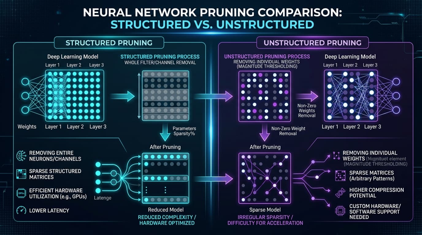
When designing a pruning strategy, practitioners face a primary architectural choice: structured vs. unstructured weight removal. Unstructured pruning removes individual weights based on importance, creating sparse matrices that are highly flexible but difficult for general-purpose processors to accelerate. Structured pruning, on the other hand, removes cohesive units like entire channels, attention heads, or layers, resulting in smaller, dense architectures that achieve direct, out-of-the-box hardware speedups on standard GPUs and edge devices.
Deploying these pruned architectures effectively requires navigating a complex design space. The choice of compression method directly impacts the hardware and software systems used, similar to how local execution frameworks operate under memory constraints as discussed in Local LLM Execution and GPU Offloading.
This article provides a rigorous comparison of structured and unstructured pruning, evaluating their underlying mechanisms, structural performance, and real-world failure modes in enterprise deployments.
What Is It?
Neural network pruning is a model compression technique that selectively removes parameters from a trained model to reduce its size and computational requirements. The fundamental premise of pruning is that deep learning models are typically over-parameterized; many weights contribute minimally to the model's final outputs. By identifying and eliminating these redundant components, we can compress the network while maintaining acceptable task performance.
The taxonomy of pruning is primarily defined by the granularity of the removed components:
Unstructured Pruning (Fine-Grained)
Unstructured pruning operates at the individual parameter level. Each weight in a weight matrix is evaluated independently based on an importance metric (usually absolute magnitude). Weights that fall below a designated threshold are set to zero. The overall dimensions of the weight matrices remain unchanged, but the matrices become sparse.
Because unstructured pruning evaluates each weight in isolation, it can achieve very high sparsity levels (e.g., 50% to 90%) with minimal impact on accuracy. The model's topology is preserved, and the zeros are scattered randomly throughout the parameter tensors.
Structured Pruning (Coarse-Grained)
Structured pruning removes entire architectural blocks from the network. Instead of targeting individual weights, it targets structural components such as channels, convolutional filters, attention heads, projection dimensions, or entire transformer layers.
When a structure is pruned, it is physically deleted from the model. This reduces the dimensions of the surrounding weight matrices. For example, pruning an attention head reduces the projection matrix sizes, and removing a layer decreases the network depth. The resulting model is smaller and composed of dense, standard-sized tensors.
Semi-Structured Pruning (NVIDIA 2:4 Sparsity)
Semi-structured pruning is a hybrid approach that enforces a specific sparsity pattern to leverage specialized hardware features. The most prominent example is NVIDIA's 2:4 semi-structured sparsity, introduced in the Ampere GPU architecture.
In this pattern, for every contiguous block of four weights in a matrix, exactly two must be pruned (set to zero). This guarantees a uniform 50% sparsity rate while adhering to a strict, regular pattern that specialized hardware cores can parse and accelerate.
Why It Matters
Model pruning addresses the primary bottlenecks of modern deep learning inference: VRAM capacity limits and memory bandwidth constraints.
The Memory Bandwidth Bottleneck
Modern LLM inference is highly memory-bandwidth bound during the autoregressive generation phase. During this step, the GPU must generate tokens one by one. For each generated token, the GPU must load the entire model's weights from High Bandwidth Memory (HBM) to its local registers to perform a single vector-matrix multiplication.
Because the compute operations per weight load are extremely low during this phase, the GPU spends most of its time waiting for memory transfers. If a model's size can be reduced by 50%, the time required to load the model parameters is halved, leading to a direct increase in inference speed (measured in tokens per second).
VRAM Capacity and Edge AI
Deploying models on resource-constrained hardware—such as edge NPUs, mobile devices, or browser-based environments using WebGPU—requires fitting the model within tight memory limits. If a model exceeds the available device memory, it cannot be run, or it must rely on slow memory swapping (e.g., system RAM offloading), which decimates performance.
Pruning allows developers to fit models onto smaller hardware footprints. For instance, structured pruning can transform a Llama-7B model into a 4B variant, enabling it to run smoothly on standard consumer devices or mid-tier enterprise servers.
How It Works
Pruning algorithms rely on different importance metrics to determine which parameters to remove. Below, we examine the primary mathematical formulations and algorithmic frameworks used.
Magnitude-Based Pruning
Traditional magnitude-based pruning uses the absolute value of the weight as a proxy for its importance. The underlying assumption is that weights with small values contribute less to the output activations.
For a weight matrix W, we define a mask M of the same shape. The pruned weight matrix W_pruned is computed as:
W_pruned = W * M
Where the mask elements M_ij are determined by:
M_ij = 1  if |W_ij| >= threshold
M_ij = 0  if |W_ij| < threshold
While magnitude pruning is computationally simple and fast, it often leads to severe accuracy degradation in modern transformer models when applied without extensive retraining. This is because it ignores the input activations, which can significantly amplify the effect of smaller weights.
Wanda (Pruning by Weights and Activations)
To address the limitations of magnitude pruning in LLMs without requiring retraining, the Wanda algorithm incorporates input activation statistics. The key insight is that LLM activations contain high-magnitude outlier features. A weight with a small magnitude can still produce a large output if it is multiplied by a highly active input feature.
Wanda evaluates weight importance on a per-output basis. For each weight W_ij connecting input j to output i, Wanda computes an importance score S_ij:
S_ij = |W_ij| * ||X_j||_2
Where ||X_j||_2 is the L2-norm of the input activations across a calibration dataset. The algorithm then prunes the weights with the lowest scores within each row of the weight matrix. Because Wanda requires only a forward pass on a small calibration set (typically 128 samples) to gather activation norms, it is extremely fast and preserves accuracy much better than raw magnitude pruning.
SparseGPT (Hessian-Based Pruning)
SparseGPT is a highly accurate, post-training unstructured pruning algorithm. It frames pruning as a local layer-wise reconstruction problem, attempting to minimize the squared error between the original layer outputs and the pruned layer outputs:
min_M || W * X - W_pruned * X ||_2^2
To solve this optimization problem efficiently, SparseGPT utilizes second-order Hessian information. The Hessian matrix H of the reconstruction loss with respect to the weights is calculated using the input activations:
H = 2 * X * X_T
SparseGPT iteratively prunes weights and adjusts the remaining unpruned weights to compensate for the introduced error. The weight update rule uses the inverse Hessian H_inv:
W_update = W - (W * M_inverse) * (H_inv / H_inv_diagonal)
By dynamically adjusting the remaining weights, SparseGPT can achieve high levels of sparsity (e.g., 50% to 60% unstructured) with near-zero loss in model perplexity, all without requiring full-parameter fine-tuning.
Structured Pruning Selection
Structured pruning requires identifying and removing entire sub-networks. This is typically done in one of three ways:
- L1-Norm Grouping: Evaluating the sum of absolute weights for a structural unit. For example, the importance of an attention head is calculated as the sum of the L1-norms of all weights within its query, key, and value projection matrices. Heads with the lowest L1-sums are removed.
- Taylor Expansion Saliency: Approximating the change in loss if a structural unit were removed. This is calculated using the gradients of the loss with respect to the activations:
WhereSaliency = | (dL / dY) * Y |Yis the output tensor of the component (e.g., the output of an attention head). - Meta-Learning and Distillation: Using a teacher-student framework to transfer knowledge from a large model to a smaller, structured pruned model. During this process, the student's architecture is initialized by pruning layers and channels from the teacher based on activation analysis, followed by continued pre-training.
Architecture
The choice of pruning method alters the physical layout of the network's parameters and computation graph.
Original Dense Matrix [4x4]      Unstructured Pruning (Sparse)   Structured Pruning (Dense)
  [ w1  w2  w3  w4 ]               [ w1   0  w3   0 ]               [ w1  w3 ]
  [ w5  w6  w7  w8 ]    ------->   [  0  w6   0  w8 ]    ------->   [ w5  w7 ]
  [ w9  w10 w11 w12]               [ w9   0  w11  0 ]               [ w9  w11]
  [ w13 w14 w15 w16]               [  0  w14  0  w16]

  (Dense operations)               (Requires sparse kernels)       (Standard dense operations)
In unstructured pruning, the tensor shapes remain identical to the original model. The zero-valued weights must be stored using specialized sparse data formats (such as Coordinate format or Compressed Sparse Row) to save storage space. However, at run time, if standard dense kernels are used, the zeros are still computed, resulting in no execution speedup.
In structured pruning, the tensor dimensions are physically reduced. For instance, if an MLP intermediate layer's projection dimension is pruned from 11,088 down to 8,256, the weight matrices are resized accordingly. The resulting model is a standard dense network that runs natively on any deep learning framework.
The following table compares the structural characteristics of these pruning granularities:
Table 1: Structural Comparison of Pruning Methods
| Feature | Unstructured Pruning | 2:4 Semi-Structured Sparsity | Structured Pruning |
|---|---|---|---|
| Granularity | Individual weight parameters | Blocks of 4 values (2 zeros) | Attention heads, channels, layers |
| Matrix State | Sparse (irregular zero patterns) | Sparse (regular 50% pattern) | Dense (smaller matrix dimensions) |
| Memory Saving | Requires compression formats | 50% index/metadata overhead | Direct reduction of tensor sizes |
| KV Cache Impact | None (hidden dimension unchanged) | None (attention heads unchanged) | Direct reduction (fewer heads/layers) |
| Topology Change | None (shapes remain constant) | None (shapes remain constant) | Yes (matrix shapes shrink) |
Production Deployment Considerations
Deploying pruned models in production requires matching the pruning style with the target hardware and software infrastructure.
Hardware Acceleration Compatibility
The primary hurdle for unstructured pruning is the lack of hardware acceleration. CPUs and GPUs are designed for high-density, parallel matrix multiplications. Irregular, scattered zeros disrupt the memory alignment and execution pathways of standard execution threads.
To achieve speedups with unstructured sparsity, one must use specialized sparse compilers or run on hardware architectures designed for sparse operations. In contrast, structured pruned models represent standard dense matrices, making them fully compatible with all existing hardware, including consumer CPUs, mobile NPUs, and GPUs.
Table 2: Hardware Acceleration Compatibility Matrix
| Hardware Platform | Unstructured Pruning | 2:4 Semi-Structured | Structured Pruning |
|---|---|---|---|
| NVIDIA Ampere/Hopper | No speedup (dense fallback) | Up to 1.8x speedup (Sparse Cores) | Direct speedup (dense operations) |
| Apple Neural Engine | No speedup | No speedup | Direct speedup |
| Edge NPUs (Qualcomm) | No speedup | No speedup | Direct speedup |
| Intel/AMD CPUs | No speedup (unless using AVX-512 sparse) | No speedup | Direct speedup |
| Consumer GPUs (RTX 30/40) | No speedup | Up to 1.5x speedup | Direct speedup |
Software Stack Integration
To deploy semi-structured 2:4 sparse models, you must use software libraries that support NVIDIA's sparse Tensor Cores, such as PyTorch's to_sparse_semi_structured API or NVIDIA's cusparSELt library.
For structured pruned models, integration is seamless. Standard inference engines like vLLM, TensorRT-LLM, and llama.cpp can run structured pruned models natively because they appear as standard models with modified dimension configurations.
This compatibility is particularly important when deploying models with optimized attention mechanisms. For example, models utilizing Grouped-Query Attention, which we compare in our guide on Mitigating Attention Bottlenecks with FlashAttention, MQA, and GQA can be structured-pruned by removing query/key/value heads in groups, preserving the GQA ratio and maintaining compatibility with high-performance kernel implementations.
Common Mistakes
Many engineering teams encounter major roadblocks when applying pruning to production systems. Below are the most common pitfalls and how to avoid them:
1. Expecting Out-of-the-Box Speedups with Unstructured Sparsity
The most common mistake is assuming that zeroing out 50% of a model's weights will make it run twice as fast. Without custom sparse inference kernels, standard deep learning libraries (like PyTorch or ONNX Runtime) will execute the sparse matrices using standard dense kernels, performing calculations on the zeros and yielding zero latency improvement. In many cases, using sparse libraries on unoptimized hardware can actually slow down inference due to the overhead of indexing sparse elements.
2. Neglecting Post-Pruning Fine-Tuning and Distillation
Pruning, even when using advanced algorithms like Wanda or SparseGPT, introduces structural disruption to the network's learned representations. Deploying a pruned model immediately after zeroing weights often leads to a severe drop in accuracy and reasoning capabilities.
To recover performance, teams must perform a phase of continued pre-training or knowledge distillation. During this phase, the pruned model (the student) is trained on a high-quality dataset while optimizing a loss function that aligns its outputs with the original unpruned model (the teacher).
3. Pruning the Wrong Layer Dimensions
In structured pruning, removing dimensions without considering hardware tensor alignment can hurt performance. Modern GPUs perform matrix operations most efficiently when tensor dimensions are multiples of 8, 16, or 32 (due to memory coalescing and thread warp sizing).
Pruning a layer's output dimension to an irregular number (e.g., 4,091 instead of 4,096) can disable optimized Tensor Core kernels, causing the GPU to fall back to slower execution paths. Always round pruned dimensions to the nearest multiple of 8 or 16.
4. Over-Pruning Sensitive Components
Certain parts of transformer architectures are highly sensitive to parameter loss. The embedding layers and the final vocabulary projection layer contain dense representations of language tokens. Pruning these layers aggressively often leads to immediate, unrecoverable perplexity collapse.
It is best practice to keep embedding and head projection layers untouched, focusing pruning efforts on the intermediate layers of the MLP Blocks and the attention projections.
Lessons From Production Deployments
Practical case studies from major AI research labs illustrate the real-world utility and recovery methodologies for structured pruning.
Case Study 1: Sheared-LLaMA (Princeton University)
The researchers behind Sheared-LLaMA demonstrated that structured pruning combined with targeted continued training is a highly effective way to create smaller, efficient models.
- Objective: Prune LLaMA-2-7B down to smaller target sizes (2.7B and 1.3B) to compete with models trained from scratch.
- Methodology: The team used structured pruning to prune the hidden dimensions, intermediate dimensions, attention heads, and layers of the 7B model. After pruning, they performed continued pre-training on 50 billion tokens.
- Results: Sheared-LLaMA-2.7B outperformed other models of similar sizes (like Pythia-2.8B and OpenLLaMA-3B) while requiring only 3% of the training compute compared to training a model of that size from scratch.
Case Study 2: NVIDIA Minitron
NVIDIA utilized structured pruning to derive smaller variants of their Llama-3.1-8B and Nemotron-4-15B models.
- Objective: Build a high-performance 4B parameter model from Llama-3.1-8B.
- Methodology: They evaluated weight saliency across the transformer layers and pruned the MLP intermediate dimension and the hidden dimension. To recover accuracy, they used knowledge distillation with the original 8B model acting as the teacher, training on a curated dataset of 94 billion tokens.
- Results: The resulting Llama-3.1-Minitron-4B retained exceptional benchmark performance, demonstrating that structured pruning is a viable alternative to training smaller models from scratch, saving millions of dollars in compute costs.
Table 3: Performance Comparison of Pruned and Base Models
| Model | Base Architecture | Parameter Count | Training Tokens (Post-Prune) | MMLU Score (5-shot) | VRAM Footprint (FP16) |
|---|---|---|---|---|---|
| LLaMA-2-7B | Base Model | 7.0 Billion | N/A (Baseline) | 45.3% | 14.0 GB |
| Sheared-LLaMA-2.7B | LLaMA-2-7B | 2.7 Billion | 50 Billion | 43.1% | 5.4 GB |
| Sheared-LLaMA-1.3B | LLaMA-2-7B | 1.3 Billion | 50 Billion | 36.8% | 2.6 GB |
| Pythia-2.8B (From Scratch) | N/A | 2.8 Billion | 300 Billion | 39.4% | 5.6 GB |
| Llama-3.1-8B | Base Model | 8.0 Billion | N/A (Baseline) | 68.4% | 16.0 GB |
| Llama-3.1-Minitron-4B | Llama-3.1-8B | 4.0 Billion | 94 Billion | 61.2% | 8.0 GB |
These deployments highlight that structured pruning is not a pure "post-training" step; it is an architecture initialization method. The true savings come from the massive reduction in pre-training tokens required to align and recover the pruned student model compared to building a model from scratch.
What Most Articles Miss
Most guides treat pruning in isolation, overlooking how it interacts with other production optimizations, specifically Quantization and KV Cache memory management.
Interaction with KV Cache and Batch Serving
In high-throughput multi-user deployment scenarios, the bottleneck is often not the model weights, but the Key-Value (KV) cache. The KV cache stores the keys and values of the self-attention layers for all active tokens in a sequence, preventing redundant computations during generation.
As discussed in our exploration of Continuous Batching and PagedAttention, managing this cache efficiently is vital for scaling concurrent requests.
Unstructured pruning does not change the hidden dimensions or the number of attention heads in the model. As a result, the size of the KV cache tensors generated for each token remains identical to the original model.
In contrast, structured pruning directly deletes attention heads and layers. Since the KV cache size is directly proportional to the number of heads and layers, structured pruning reduces the KV cache footprint by the exact ratio of the pruned components.
For instance, pruning 25% of the attention heads in a model directly frees up 25% of the VRAM allocated to the KV cache, allowing the serving system to accommodate larger batch sizes and increase throughput.
Pruning and Quantization Compatibility
When preparing a model for production, teams often want to combine pruning and quantization to achieve maximum compression. However, these two techniques can conflict if applied in the wrong order.
If a model is pruned using unstructured pruning (leaving many isolated zero weights) and then quantized using algorithms like GPTQ or AWQ, the zero values can distort the quantization scale factors. Quantization algorithms calculate scale factors based on the range of weights in a tensor block.
The presence of many absolute zeros shifts the distribution, causing the quantization step to introduce larger rounding errors on the remaining active weights, leading to accuracy collapse.
To mitigate this, developers should:
- Prune first, then quantize: Perform structured pruning and complete the recovery distillation phase to stabilize the model's weights. Once the pruned model is stable and dense, apply post-training quantization.
- Use Joint Optimization: If using semi-structured 2:4 sparsity, use frameworks (like TensorRT-LLM) that support joint sparse-quantized operations, where the sparse mask is applied during the quantization scale calculation to prevent distortion.
Best Practices
To build a robust model optimization pipeline, follow these guidelines:
- Prioritize Structured Pruning for Standard Hardware: If you are deploying on standard CPUs, edge devices, or standard GPU instances without dedicated sparse kernels, use structured pruning. It guarantees hardware-independent speedups.
- Use Wanda for Rapid Heuristic Evaluation: When evaluating different target sizes on a tight timeline, use Wanda. It is fast, requires no weight updates, and provides a clear picture of how sensitive different layers are to pruning.
- Incorporate Knowledge Distillation: Always pair structured pruning with a post-pruning distillation phase. Use the original unpruned model as the teacher to guide the pruned student, training on high-quality domain data to recover accuracy.
- Align Dimensions with Hardware Layouts: Ensure that all pruned layers are rounded to multiples of 8 or 16. This preserves alignment with GPU warps and Tensor Core execution requirements.
- Protect Critical Layers: Keep embedding layers, positional encoding layers, and final output heads untouched. Focus pruning on the internal MLP intermediate projections and self-attention projections.
- Sequence Optimizations Correctly: Run structured pruning first, followed by continued training to stabilize weights, and perform quantization as the final step.
FAQ
1. Does unstructured pruning reduce model file size?
Yes, but only if the model is saved using a sparse storage format (such as CSR or COO) or compressed (e.g., using gzip). If saved as a standard dense tensor, the zero values still occupy the same storage space as non-zero parameters.
2. Why is structured pruning preferred over unstructured pruning?
Structured pruning physically removes parameters and resizes tensors, converting the model into a standard, smaller dense network. This allows it to run faster on any standard hardware without requiring specialized sparse execution engines.
3. What is NVIDIA's 2:4 semi-structured sparsity?
It is a hardware-supported sparsity pattern where in every block of 4 weights, exactly 2 must be zero. NVIDIA Ampere and Hopper GPUs contain dedicated Tensor Core instructions that skip calculations on these zeros, doubling theoretical math throughput.
4. How does pruning interact with KV cache size?
Structured pruning reduces the KV cache size because it deletes attention heads or layers, which directly shrinks the active memory required for key-value projections during serving. Unstructured pruning has no effect on KV cache size.
5. Should I prune or quantize my model first?
You should prune first. Pruning reduces the tensor sizes and structural configuration. Once the model's weights are stabilized and distilled, you can apply quantization. Quantizing before pruning makes it extremely difficult to perform weight updates and fine-tuning.
6. Can I recover all the accuracy lost during pruning?
With moderate pruning ratios (e.g., pruning 10% to 20% of layers or channels), you can often recover nearly 100% of the baseline accuracy using knowledge distillation. At higher compression ratios, some accuracy loss is expected, but it is significantly less than that of un-distilled models.
7. What is the Wanda pruning algorithm?
Wanda (Weights and activations) is a post-training pruning algorithm that evaluates weight importance by multiplying weight magnitudes by the L2-norm of their input activations. This allows it to identify and preserve weights that interact with high-amplitude activation features.
8. What is SparseGPT?
SparseGPT is a post-training pruning algorithm that uses second-order Hessian information to prune weights and dynamically adjust the remaining weights to minimize reconstruction error, allowing for high sparsity with minimal accuracy loss.
9. Does pruning work on Convolutional Neural Networks (CNNs)?
Yes. In CNNs, structured pruning typically removes entire convolutional channels or filters, which reduces the width of subsequent feature maps, leading to direct latency improvements.
10. How many training tokens are needed to recover a pruned model?
Depending on the size of the model and the pruning ratio, recovery typically requires between 10 billion and 100 billion tokens. While this represents a significant computational effort, it is still a small fraction (e.g., 3% to 5%) of the tokens required to train an equivalent model from scratch.
Key Takeaways
- Hardware Support is Critical: Unstructured pruning is highly flexible but provides no latency benefits on standard hardware without specialized sparse kernels. Structured pruning is universally compatible and delivers immediate speedups.
- Structured Pruning Shrinks KV Cache: By removing attention heads and layers, structured pruning directly reduces the VRAM allocated to the KV cache, enabling larger batch sizes during concurrent serving.
- Sequence Matters: When combining compression techniques, always prune and distill the model before applying quantization to prevent scale distortions and accuracy collapse.
- Recovery Requires Distillation: Pruning must be viewed as an architecture initialization step. Running continued pre-training or knowledge distillation using the base model as a teacher is essential to recover accuracy.
- Target the Internal Layers: Keep embedding layers and output projection layers untouched, focusing parameter removal on the wide MLP intermediate dimensions and attention projection layers.