Mitigating Attention Bottlenecks: FlashAttention, Multi-Query Attention (MQA), and GQA
How modern LLM architectures optimize KV cache memory bandwidth during long-context decoding.

In the rapid evolution of large language models (LLMs), scaling context windows from 2K to 128K, 1M, or even more tokens has transitioned from an experimental feature to a core requirement. However, this expansion exposes a critical bottleneck in the underlying Transformer architecture: the Key-Value (KV) cache.
During the autoregressive decoding phase—where an LLM generates text one token at a time—the attention mechanism needs to access the Key and Value vectors of all previous tokens. Storing these vectors prevents redundant calculations but introduces a massive memory overhead that scales linearly with sequence length and batch size. This makes LLM serving highly memory-bound rather than compute-bound.
To address this "memory wall," the AI research community has developed two complementary classes of optimizations:
- Architectural Optimizations: Changing the model structure itself during training to compress the size of the KV cache. This is where Multi-Query Attention (MQA) and Grouped-Query Attention (GQA) reside.
- Algorithmic and Hardware Co-design: Changing how attention is computed on hardware without changing the mathematical output of the attention equation. This is the domain of FlashAttention (and its iterations FlashAttention-2, 3, and 4).
This article provides a deep architectural and mathematical dive into how FlashAttention, MQA, and GQA function, how they interact with serving infrastructures like vLLM and TensorRT-LLM, and how to configure them for high-throughput, low-latency production deployments.
🧱 What Is It?
To understand these optimizations, we must first define the baseline attention mechanism: Multi-Head Attention (MHA).
Multi-Head Attention (MHA)
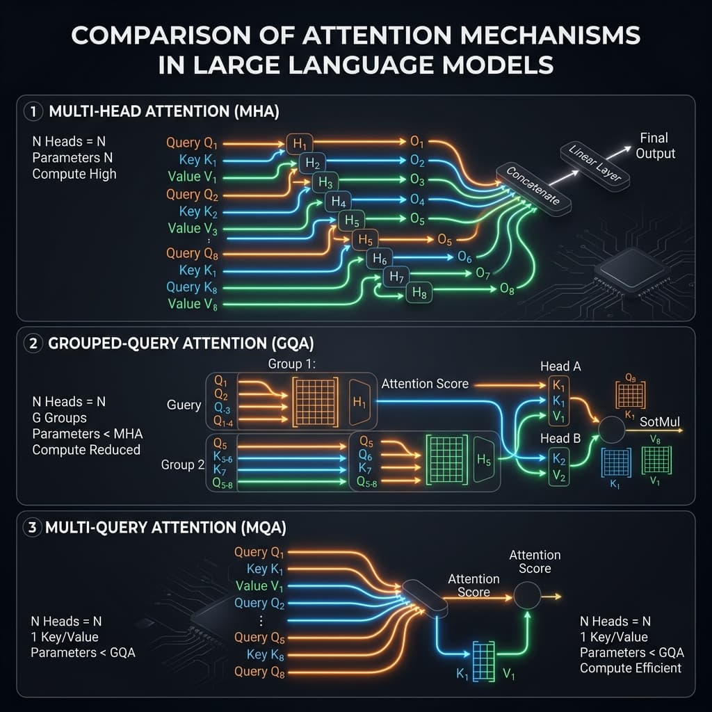
In standard Multi-Head Attention (MHA), every query head (Q) has a corresponding, dedicated key head (K) and value head (V). If a model has H_q query heads, it also has H_k = H_q key heads and H_v = H_q value heads. For example, Llama 2 70B uses 64 query heads and 64 key/value heads. This one-to-one mapping ensures maximum expressivity but results in a massive KV cache because every single head generates and stores unique Key and Value vectors for every token in the sequence.
Multi-Query Attention (MQA)
Introduced by Noam Shazeer in 2019, Multi-Query Attention (MQA) is a radical architectural modification. In MQA, there is only one key head and one value head shared across all query heads. That is, H_k = H_v = 1, while H_q remains large (e.g., 32 or 64).
By consolidating the key and value heads, MQA reduces the memory footprint of the KV cache by a factor equal to the number of query heads (e.g., a 32x or 64x reduction). However, this aggressive compression can degrade model quality and semantic capacity because the model has less capacity to represent diverse relationships per token across different heads.
Grouped-Query Attention (GQA)
Grouped-Query Attention (GQA), introduced in 2023, is the modern compromise. Instead of sharing one KV head across all query heads (MQA) or having a unique KV head for every query head (MHA), GQA groups query heads into G groups. Each group shares a single key and value head.
For example, if a model has 32 query heads and is grouped into 8 groups, each group contains 4 query heads sharing 1 key and 1 value head (H_k = H_v = 8, grouping ratio H_q / H_k = 4). GQA offers a tunable parameter that allows architects to balance accuracy and memory footprint. It has become the standard for modern frontier architectures like Llama 3, Qwen 2, and Mistral.
FlashAttention
Unlike MQA and GQA, FlashAttention does not change the attention architecture or the mathematical output. It is a hardware-aware, I/O-conscious implementation of the standard attention equation.
Typically, computing attention requires materializing a massive intermediate matrix of size N \times N (where N is the sequence length) to hold attention scores. Writing and reading this matrix to and from the GPU's High Bandwidth Memory (HBM) is incredibly slow. FlashAttention uses tiling, online softmax, and recomputation during the backward pass to compute exact attention without ever writing the N \times N matrix to HBM, keeping the computations inside the GPU’s ultra-fast SRAM.
⚡ Why It Matters
To understand why these optimizations are critical, we must look at the transition between the two phases of LLM inference: Prefill and Decode.
+---------------------------------------------------------------------------------+
|                               LLM INFERENCE PHASES                              |
+---------------------------------------+-----------------------------------------+
|                PREFILL                |                  DECODE                 |
|  - Process prompt tokens in parallel  |  - Generate output tokens sequentially  |
|  - Compute-bound (matrix multiplies)  |  - Memory-bound (loading KV cache)      |
|  - High GPU Tensor Core utilization   |  - Limited by memory bandwidth (HBM)    |
+---------------------------------------+-----------------------------------------+
The Compute vs. Memory Bound Paradigm
In GPU computation, algorithms are classified based on their Arithmetic Intensity—the ratio of floating-point operations (FLOPs) performed per byte of data transferred from VRAM (HBM).
- Compute-bound: The processing speed is limited by the GPU's raw compute power (Tensor Cores). The Prefill phase is compute-bound because all prompt tokens are processed in parallel, allowing massive matrix-matrix multiplications (
GEMM) that fully saturate Tensor Cores. - Memory-bound: The processing speed is limited by how fast data can be read from and written to memory (VRAM to SRAM). The Decode phase is memory-bound because we process only one token at a time. For each generated token, the GPU must load all model weights AND the entire historical KV cache from HBM to compute attention.
On an H100 GPU, memory bandwidth is approximately 3.35 TB/s, while compute performance is 989 TFLOPs (FP16). If the arithmetic intensity of a kernel is low, the compute units sit idle, waiting for data to arrive from VRAM. This is known as the Memory Wall.
The KV Cache Memory Wall
The memory consumption of the KV cache scales according to the following equation:
KV Cache Size (Bytes) = 2 * Batch Size (B) * Sequence Length (L) * KV Heads (H_kv) * Head Dim (D) * Precision (P)
Where:
2: Represents the two matrices (Key and Value).B: Batch size (number of parallel requests).L: Sequence length (context window).H_{kv}: Number of KV heads.D: Head dimension (typically 128).P: Precision in bytes (2 bytes for FP16/BF16, 1 byte for FP8/INT8).
Let's calculate the memory required for the KV cache of a model using MHA (e.g., Llama 2 7B, where H_q = H_k = 32, D = 128) at FP16 precision (P = 2) with a batch size of 64 and a context length of 4096 tokens:
MHA Size = 2 * 64 * 4096 * 32 * 128 * 2 = 4,294,967,296 bytes ≈ 4.29 GB
Compare this with a GQA-enabled model (e.g., Llama 3 8B, where H_q = 32 but H_{kv} = 8, grouping ratio of 4):
GQA Size = 2 * 64 * 4096 * 8 * 128 * 2 = 1,073,741,824 bytes ≈ 1.07 GB
And with an MQA-enabled model (H_kv = 1):
MQA Size = 2 * 64 * 4096 * 1 * 1 * 128 * 2 ≈ 134.2 MB
By moving from MHA to GQA, we achieve a 75% reduction in KV cache memory footprint, and with MQA, a 96.8% reduction. This directly translates to:
- Higher Batch Sizes: Allowing the system to serve 4x more concurrent users on the same GPU.
- Longer Contexts: Serving inputs that are 4x longer before running out of memory (OOM).
- Lower Latency: Reducing the amount of data transferred from HBM, which accelerates the memory-bound decoding phase.
🛠️ How It Works
The Mechanics of MQA and GQA
MQA and GQA compress the KV cache by altering the projection matrices of the Transformer layer.
In standard MHA, the input tensor X of shape $[B, L, D_]$ is multiplied by three projection matrices: W_Q, W_K, and W_V to generate query, key, and value representations.
MHA:
Q Heads: [H_q]   ==>  [Q1] [Q2] [Q3] [Q4] ... [Q32]
KV Heads: [H_kv] ==>  [K1] [K2] [K3] [K4] ... [K32] (Each query head has its own KV head)

MQA:
Q Heads: [H_q]   ==>  [Q1] [Q2] [Q3] [Q4] ... [Q32]
KV Heads: [H_kv] ==>  [K1]                        (All query heads share a single KV head)

GQA:
Q Heads: [H_q]   ==>  [Q1 Q2 Q3 Q4]  [Q5 Q6 Q7 Q8]  ... [Q29 Q30 Q31 Q32]
KV Heads: [H_kv] ==>  [   KV1    ]  [   KV2    ]  ... [     KV8     ] (Groups of queries share a KV head)
In GQA, the projection weights W_K and W_V are configured to output a smaller dimension. Instead of mapping to H_q * D_head, they map to H_kv * D_head, where H_kv = H_q / group_ratio. During the attention computation, the Key and Value states are replicated or broadcasted across the query heads within their group, allowing standard dot-product attention to proceed.
The Inner Workings of FlashAttention
Standard attention computation follows the classic softmax formula:
Attention(Q, K, V) = softmax( (Q * K^T) / sqrt(d_k) ) * V
To calculate this naively:
- Load
QandKfrom HBM to SRAM. - Compute
S = QK^T(sizeN \times N, stored in HBM). - Load
Sfrom HBM, computeP = \text{softmax}(S)(sizeN \times N, stored in HBM). - Load
PandVfrom HBM, computeO = PV(sizeN \times d, stored in HBM).
This requires reading and writing the N \times N matrix (S and P) multiple times. For a context length of 100K, the N \times N matrix contains 10^{10} elements, requiring 20 GB of memory just to store the intermediate attention scores!
NAIVE ATTENTION (Memory-bound due to HBM reads/writes):
[HBM] --(Load Q,K)--> [SRAM] --(Compute QK^T)--> [HBM (Store N x N)] --(Load N x N)--> [SRAM] --(Compute Softmax)--> [HBM (Store Softmax)] --(Load Softmax, V)--> [SRAM] --(Compute O)--> [HBM]

FLASHATTENTION (Tiled, IO-aware, all compute in SRAM):
[HBM] --(Load Q, K, V in tiles)--> [SRAM (Block-wise compute, online softmax, partial outputs)] --(Output O)--> [HBM]
FlashAttention avoids this HBM transfer using three techniques:
1. Tiling (Block-wise Computation)
FlashAttention splits the inputs Q, K, and V into blocks (tiles) that fit into the GPU’s fast SRAM (which is only a few tens of megabytes, e.g., 228 KB per Streaming Multiprocessor on H100). The attention computation is performed block-by-block.
2. Online Softmax
Standard softmax requires knowing the maximum value of the entire row to compute the denominator (\sum e^{x_i - x_{max}}). When computing in blocks, we do not have access to the entire row at once. FlashAttention uses a mathematical trick to compute softmax incrementally (online).
If we have a block's partial softmax and load a new block, we can rescale the old block's output using the new running maximum and sum of exponentials, yielding mathematically identical results:
m_new = max(m_old, m_block)
s_new = s_old * exp(m_old - m_new) + s_block * exp(m_block - m_new)
O_new = diag(exp(m_old - m_new)) * O_old * (s_old / s_new) + (P_block * V_block) / s_new
3. Recomputation in Backward Pass
During backpropagation, standard attention loads the intermediate N \times N softmax matrix from HBM. FlashAttention avoids storing this by recomputing the softmax block-by-block on the fly during the backward pass. Recomputing is significantly faster than reading the massive matrix from HBM because compute (ALUs/Tensor Cores) is much faster than memory bandwidth.
🏗️ Architecture
Let's examine how MHA, GQA, and MQA compare structurally.
Table 1: Structural and Operational Comparison
| Feature / Dimension | Multi-Head Attention (MHA) | Grouped-Query Attention (GQA) | Multi-Query Attention (MQA) |
|---|---|---|---|
KV Head Count (H_kv) | Equal to Query Heads (H_{kv} = H_q) | H_{kv} = H_q / \text{ratio} (typically 4 or 8) | Single Head (H_kv = 1) |
| KV Cache Footprint | Baseline (100% size) | Compressed (12.5% to 25% of MHA) | Maximum Compression (1.5% to 3% of MHA) |
| Accuracy / Quality | Baseline (Highest) | Very close to MHA (often $\ge 99%$) | Noticeable degradation in complex tasks |
| Training Stability | High | High | Moderate (requires careful tuning) |
| Decode Throughput | Low (highly memory-bound) | High | Maximum |
| Standard Use Case | Legacy Models (e.g., Llama 1) | Modern Frontier LLMs (Llama 3, Mistral) | Edge / Highly Latency-Critical Models |
Mathematical Scaling of Popular Architectures
To illustrate the difference in real-world systems, let's analyze the KV cache size scaling for different configurations of popular LLMs.
Table 2: KV Cache Memory Footprint per Token (in Bytes)
| Model Name | Parameter Size | Attention Type | Query Heads | KV Heads | Head Dim | FP16 Cache (Bytes/Token) | FP8 Cache (Bytes/Token) | 32k Context Cache (FP16, B=64) |
|---|---|---|---|---|---|---|---|---|
| Llama 2 7B | 7B | MHA | 32 | 32 | 128 | 16,384 | 8,192 | 33.55 GB |
| Llama 3 8B | 8B | GQA | 32 | 8 | 128 | 4,096 | 2,048 | 8.38 GB |
| Mistral 7B | 7B | GQA | 32 | 8 | 128 | 4,096 | 2,048 | 8.38 GB |
| Gemma 2 9B | 9B | GQA | 16 | 8 | 256 | 8,192 | 4,096 | 16.78 GB |
| Llama 3 70B | 70B | GQA | 64 | 8 | 128 | 4,096 | 2,048 | 8.38 GB |
| Falcon 40B | 40B | MQA | 64 | 1 | 64 | 256 | 128 | 0.52 GB |
Note: The table highlights how Llama 3 70B, despite its massive size, has the exact same KV cache footprint as Llama 3 8B because they both use 8 KV heads with a head dimension of 128!
⚡ Production Deployment Considerations
Deploying these architectures in high-scale serving environments (like vLLM, Triton, or TensorRT-LLM) requires addressing several secondary bottlenecks.
1. PagedAttention
Traditional KV cache management allocates a contiguous block of VRAM for the maximum possible sequence length of a request (e.g., reserving space for 4096 tokens even if the request only generates 100 tokens). This leads to External and Internal Memory Fragmentation, wasting up to 60–80% of available memory.
CONTIGUOUS ALLOCATION (High waste):
| Request 1 (Reserved for 4K tokens) [Used: 200] [Wasted: 3800] | Request 2 (Reserved for 4K) [Used: 50] |

PAGEDATTENTION (Virtual memory style):
| Block Page 1 (16 tokens) | Block Page 99 (16 tokens) | Block Page 3 (16 tokens) | Block Page 12 (16 tokens) |
(Dynamically allocated, non-contiguous physical memory, zero fragmentation)
PagedAttention solves this by borrowing the concept of virtual memory and paging from operating systems. It divides the KV cache into fixed-size physical memory pages (blocks, typically 16 or 32 tokens). When a token is generated, the engine maps logical tokens to non-contiguous physical pages. This eliminates fragmentation, reducing memory waste to less than 4%, allowing serving systems to double or triple their concurrent batch sizes.
2. FlashDecoding: Parallelizing the Decode Phase
While FlashAttention optimizes the compute-bound prefill phase (parallelized over query length), it loses efficiency during the sequential decode phase. In decoding, the query length is 1 (N_query = 1), while the key-value sequence length is large (N_kv >= 100,000). Standard FlashAttention parallelizes work over the Batch Size and Query Head dimensions. If the batch size is small, only a few Streaming Multiprocessors (SMs) on the GPU are utilized, leaving the rest of the GPU idle.
FlashDecoding solves this by parallelizing the attention computation across the sequence length of the KV cache (the split-K approach):
- It splits the long KV cache into multiple blocks.
- It computes the attention scores and partial outputs for each block in parallel using multiple SMs.
- It performs a final reduction step to combine the partial outputs using online softmax scaling.
This achieves a 10x speedup in decoding for sequence lengths above 32K tokens.
FLASHDECODING SPLIT-K FLOW:
                     +---------------------------------------+
                     |             User Query                |
                     +-------------------+-------------------+
                                         |
            +----------------------------+----------------------------+
            |                            |                            |
  [KV Cache Block 1]           [KV Cache Block 2]           [KV Cache Block 3]
  (Process on SM 1)            (Process on SM 2)            (Process on SM 3)
            |                            |                            |
    [Partial Output 1]           [Partial Output 2]           [Partial Output 3]
            +----------------------------+----------------------------+
                                         |
                                         v
                     +---------------------------------------+
                     |        Softmax Reduction (SM 4)       |
                     +-------------------+-------------------+
                                         v
                                   [Final Output]
3. KV Cache Quantization (FP8 and INT8/INT4)
To squeeze even more performance out of memory-bound systems, serving engines support quantizing the KV cache to FP8, INT8, or INT4.
-
FP8 KV Cache: Uses 8-bit floating-point formats (E4M3 or E5M2). E4M3 offers better precision for activations, making it ideal for the KV cache. Quantization to FP8 halves the memory requirement of the KV cache with almost zero degradation in model perplexity.
-
INT8/INT4 Quantization: Quantizes vectors to integers. This requires maintaining scaling factors per channel or per block:
X_quant = round(X / scale)
    While INT4 reduces memory by 75% compared to FP16, it can introduce significant precision loss, especially in long context windows where outlier activations in the Key and Value matrices become prominent.

---

## ⚠️ Common Mistakes

When optimizing Transformer serving, engineers frequently make the following design and deployment errors:

### 1. Assuming FlashAttention Changes Model Output
FlashAttention is mathematically exact. It does not introduce approximations or alter the output of the attention mechanism (unlike GQA/MQA, which compress the representation). Running a model with FlashAttention yields the same output activations as standard attention. If you encounter quality loss after enabling FlashAttention, it is due to a buggy kernel implementation or numerical precision overflows in intermediate accumulators, not the algorithm itself.

### 2. Mismatched GQA Head Groups during Tensor Parallelism
When splitting a GQA model across multiple GPUs using Tensor Parallelism (TP), the number of KV heads must be cleanly divisible by the TP degree.
For example, Llama 3 8B has 8 KV heads. If you split it across 8 GPUs (`TP = 8`), each GPU gets exactly 1 KV head (with 4 Query heads). This works perfectly.
However, if you attempt to run Llama 3 8B with `TP = 16` or `TP = 3`, the heads cannot be split evenly, causing compilation failures or requiring slow communication overlays (all-gather) that negate GQA's latency benefits.

### 3. Neglecting the Block Size in PagedAttention
Setting the block size (number of tokens per block) too low or too high can hurt performance:
*   **Too low (e.g., 4 or 8 tokens):** Increases the size of the block allocation table, leading to high CPU overhead when managing metadata page lookups. It also prevents the GPU from coalescing memory reads efficiently.
*   **Too high (e.g., 128 or 256 tokens):** Re-introduces memory fragmentation, as the tail of a request's sequence is highly likely to leave a large portion of the final block empty.
*   **Optimal:** A block size of **16** or **32** is the industry sweet spot.

---

## 👥 Lessons From Production Deployments

Deploying LLMs at scale in production environments (serving millions of requests daily) has revealed several critical engineering constraints:

### 1. The Prefill/Decode Scheduling Conflict
Prefill operations (high compute, low memory transfer) and Decode operations (low compute, high memory transfer) compete for the same hardware resources. In naive serving setups, a new incoming request triggers a prefill phase that pauses the ongoing decode phase of existing requests, leading to high jitter and spikes in Time Per Output Token (TPOT).
Production systems use **Continuous Batching** (iteration-level scheduling) paired with **Chunked Prefills**. Instead of processing a massive prompt prefill in a single step, the prompt is divided into chunks (e.g., 512 tokens) and processed alongside decoding steps, smoothing out latency spikes.

### 2. KV Cache Eviction vs. Offloading
At massive contexts (e.g., 100K+), even GQA and FP8 cache optimization cannot prevent the KV cache from consuming the entire VRAM of a system. When VRAM is exhausted, engines must choose between:
*   **Offloading:** Swapping KV cache pages to CPU host memory via PCIe. This introduces massive latency bottlenecks when those pages must be retrieved for attention computation.
*   **Eviction (Smart Caching):** Throwing away less important KV tokens. Recent techniques (like H2O or Heavy-Hitter Oracle) identify that a small fraction of tokens (e.g., punctuation, structural words, or highly attended terms) contribute to 95% of attention weight. Evicting the remaining tokens reduces cache size dynamically without requiring slow PCIe swaps.

---

## 🔍 What Most Articles Miss

Most high-level articles explain FlashAttention as "it uses SRAM," but they omit the actual engineering challenges solved by its latest iterations, specifically **FlashAttention-3** and **FlashAttention-4**.

### Pipelining and Asynchrony in Modern Architectures
The release of NVIDIA's Hopper (H100) and Blackwell (B200) architectures introduced hardware features designed to bypass register-file bottlenecks:
*   **Hopper's TMA (Tensor Memory Accelerator):** In older GPUs (like A100), moving data from HBM to shared memory (SRAM) required registers. This created a register pressure bottleneck. Hopper's TMA allows direct, asynchronous transfer of multidimensional tensors from HBM to SRAM without involving GPU registers or execution pipelines.
*   **Blackwell's Asymmetric Scale:** Blackwell features asymmetric compute and memory execution pipelines.

Standard FlashAttention-2 does not exploit these asynchronous hardware features, causing the GPU's Tensor Cores to wait while the TMA transfers data.

**FlashAttention-3** and **FlashAttention-4** solve this by co-designing the algorithm with the hardware's pipelining structures:
1.  **Warp-Group Partitioning:** They partition the Streaming Multiprocessor (SM) warps into producer and consumer groups. The producers handle asynchronous data loading (using Hopper's TMA or Blackwell's transfer pipes), while the consumers execute GEMM operations on Tensor Cores.
2.  **Double/Triple Buffering:** They allocate multiple SRAM buffers. While the consumers execute attention math on Buffer `A`, the producers load the next tiles of `K` and `V` into Buffer `B` in parallel.
3.  **Low-Precision Accumulation (FP8):** Standard FP8 matrix multiplies can overflow easily. FlashAttention-3/4 implements block-wise scaling and specialized registers to execute accumulate operations in FP32 precision while storing inputs in FP8, maintaining exact mathematical precision.

### Table 3: Evolution of FlashAttention Implementations

| Metric / Feature | FlashAttention-1 (2022) | FlashAttention-2 (2023) | FlashAttention-3 (2024) | FlashAttention-4 (2026) |
| :--- | :--- | :--- | :--- | :--- |
| **Primary GPU Target** | Ampere (A100), Turing | Ampere, Ada Lovelace | Hopper (H100) | Blackwell (B200) |
| **Data Transfer** | Synchronous HBM `\leftrightarrow` SRAM | Optimized work partitioning | Asynchronous via TMA (Hopper) | Pipelined Asymmetric scaling |
| **Warp Structure** | Unified warps | Separated thread blocks | Producer/Consumer Warp Groups | Asymmetric execution groups |
| **FP8 Support** | No | Experimental | Native (with block scaling) | Optimized (with hardware scaling) |
| **Speedup (vs. Naive)** | 2x - 4x | 4x - 6x | 6x - 8x | 8x - 12x |

---

## 🎯 Best Practices

When deploying large language models, follow these guidelines to maximize throughput and minimize latency:

1.  **Prioritize GQA Models:** Avoid MHA models (like Llama 1) for production deployments. Choose architectures designed with GQA (e.g., Llama 3, Mistral, Qwen) to reduce memory overhead from the start.
2.  **Enable FP8 KV Cache:** In vLLM or TensorRT-LLM, configure the serving engine to use FP8 precision for the KV cache. This provides a 2x memory reduction with virtually zero impact on output quality.
3.  **Tune the PagedAttention Block Size:**
    *   Set the block size to **16** for short-context, latency-sensitive applications.
    *   Set the block size to **32** for long-context (32K+), high-throughput applications to reduce CPU-side page table overhead.
4.  **Use FlashDecoding for Long Contexts:** When sequence lengths exceed 16K tokens, ensure FlashDecoding (or split-K attention) is enabled in your framework. This prevents the decode phase from bottlenecking on a single SM.
5.  **Utilize Chunked Prefill:** For applications with long system prompts (e.g., agents or multi-document QA), configure a chunked prefill size (e.g., `chunked_prefill_size=512` in vLLM) to prevent prefill steps from stalling active decode queues.
6.  **Enforce Divisible Tensor Parallelism:** Always configure the Tensor Parallelism degree (`TP`) so that the model's KV head count (`H_kv`) is divisible by `TP` (`H_kv % TP == 0`).

For instance, here is an example configuration script using the `vllm` library to run a GQA model with FP8 KV cache and chunked prefill:

```python
from vllm import LLM, SamplingParams

# Configure optimal serving settings for Llama-3-8B-Instruct
llm = LLM(
    model="meta-llama/Meta-Llama-3-8B-Instruct",
    gpu_memory_utilization=0.90,
    max_model_len=16384,
    enable_chunked_prefill=True,
    kv_cache_dtype="fp8",         # Enable FP8 KV Cache
    block_size=16,                # Block size for PagedAttention
    tensor_parallel_size=1        # Match KV head constraints
)

sampling_params = SamplingParams(
    temperature=0.7,
    top_p=0.9,
    max_tokens=512
)
🙋 FAQ
1. What is the difference between FlashAttention, MQA, and GQA?
MQA and GQA are architectural alterations to the model's weights and structural layers that reduce the number of key/value heads, compressing the cache size. FlashAttention is an algorithmic optimization of the attention math that reduces slow VRAM reads/writes on GPU hardware without changing the mathematical output.
2. Does FlashAttention reduce the size of the KV cache?
No. FlashAttention optimizes the execution speed and hardware memory access patterns during the attention computation. The physical size of the KV cache stored in VRAM remains the same. To reduce the KV cache size, you must use GQA, MQA, or KV cache quantization.
3. Can I use FlashAttention and GQA together?
Yes, they are orthogonal and complementary. GQA reduces the size of the tensors in the KV cache, and FlashAttention speeds up the mathematical operations performed on those tensors. Modern inference engines use both simultaneously.
4. Why is MQA not used in all LLMs if it saves the most memory?
MQA reduces the key/value heads to a single head. This extreme compression removes too much capacity for representing complex relational dependencies. GQA is preferred because it restores almost all of standard MHA's modeling quality while retaining the majority of MQA's memory savings.
5. What is the difference between FlashAttention and FlashDecoding?
FlashAttention is optimized for the prefill phase (processing a batch of prompts parallelly), which has a query length N_q \ge 1. FlashDecoding is a separate kernel optimized for the decode phase (generating tokens one-by-one), where N_q = 1 and the KV cache is long. FlashDecoding parallelizes the computation across the sequence length of the KV cache (split-K).
6. Does FP8 KV cache degrade LLM performance?
In most production benchmarks, FP8 quantization of the KV cache (especially using the E4M3 format) shows negligible loss in perplexity and downstream task accuracy (often less than 0.1%), while doubling serving capacity.
7. What is memory fragmentation in the KV cache?
In standard serving, VRAM is allocated contiguously based on the maximum context length of a model (e.g., reserving space for 4096 tokens). If the request finishes early or is shorter, the unused space remains locked and cannot be shared. PagedAttention solves this by allocating memory dynamically in non-contiguous 16-token pages.
8. Why do we need chunked prefill?
When a large prompt arrives, processing it (prefill phase) takes a long time and hogs GPU compute. This stalls the generation (decode phase) of already active requests, leading to latency spikes. Chunked prefill breaks the prompt into smaller pieces, allowing prefill and decode phases to run concurrently.
9. What hardware is required for FlashAttention-3 and 4?
FlashAttention-3 requires NVIDIA Hopper GPUs (H100/H200) to utilize the asynchronous Tensor Memory Accelerator (TMA). FlashAttention-4 targets NVIDIA Blackwell GPUs (B200) to capitalize on the asymmetric compute pipelines.
10. How do I calculate the KV cache size for my model?
Multiply: 2 \times \text{Batch Size} \times \text{Sequence Length} \times \text{KV Head Count} \times \text{Head Dimension} \times \text{Byte Precision}. Divide the final number of bytes by 1,073,741,824 to get the size in Gigabytes (GB).
🎯 Key Takeaways
- KV Cache is the Bottleneck: During LLM decoding, loading the KV cache from VRAM is the primary memory bandwidth bottleneck limiting performance and batch capacity.
- GQA is the Industry Standard: Grouped-Query Attention is the default choice for modern LLMs because it compresses the KV cache footprint by 75% or more compared to MHA while maintaining equivalent model accuracy.
- FlashAttention Avoids the Memory Wall: FlashAttention speeds up computation by tiling attention matrices, computing softmax online, and avoiding slow HBM reads/writes of intermediate
N \times Nmatrices. - FlashDecoding Parallelizes Space: FlashDecoding optimizes long-context decoding by splitting the KV cache along the sequence length dimension and computing partial attention scores in parallel across multiple GPU cores.
- PagedAttention Eliminates Waste: PagedAttention structures the KV cache like operating system virtual memory pages, reducing physical memory fragmentation from over 60% down to less than 4%.
- Hardware Co-design is Essential: The latest iterations (FlashAttention-3 and FlashAttention-4) target Hopper and Blackwell GPU features like TMA, asynchronous pipelining, and FP8 accumulator registers to maximize hardware efficiency.
