Quantization Mathematics: GPTQ vs AWQ vs GGUF/GGML
A deep dive into sub-8-bit quantization techniques, activation scaling, and hardware support.

In the commercial deployment of large language models (LLMs), the transition from model training to inference serving marks a fundamental shift in engineering priorities. During training, workloads are highly compute-bound, dominated by massive, predictable matrix multiplications that keep GPU Tensor Cores fully saturated. In contrast, LLM inference serving—particularly during the token generation phase—is notoriously memory-bound, constrained by the throughput of High Bandwidth Memory (HBM) rather than raw FLOPS.
As explored in our deep dives on Mitigating Attention Bottlenecks and Continuous Batching vs PagedAttention, the autoregressive nature of LLM generation requires the system to process text one token at a time. For every generated token, the model must access the Key and Value vectors of all previous tokens. While solutions like PagedAttention and Grouped-Query Attention (GQA) reduce the size of the Key-Value (KV) cache, the model weight parameters themselves represent the single largest VRAM overhead.
For instance, a 70-billion parameter model in 16-bit precision requires 140 GB of memory just to load into VRAM. This makes it impossible to serve on a single H100 or A100 GPU without quantization. To address this "memory wall," the AI research community has developed Post-Training Quantization (PTQ) techniques.
This guide provides a rigorous mathematical and architectural breakdown of the three primary PTQ formats in modern AI engineering: GPTQ, AWQ, and GGUF/GGML. We will examine their underlying mathematics, hardware targets, dequantization overheads, and practical deployment configurations.
🧱 What Is It?
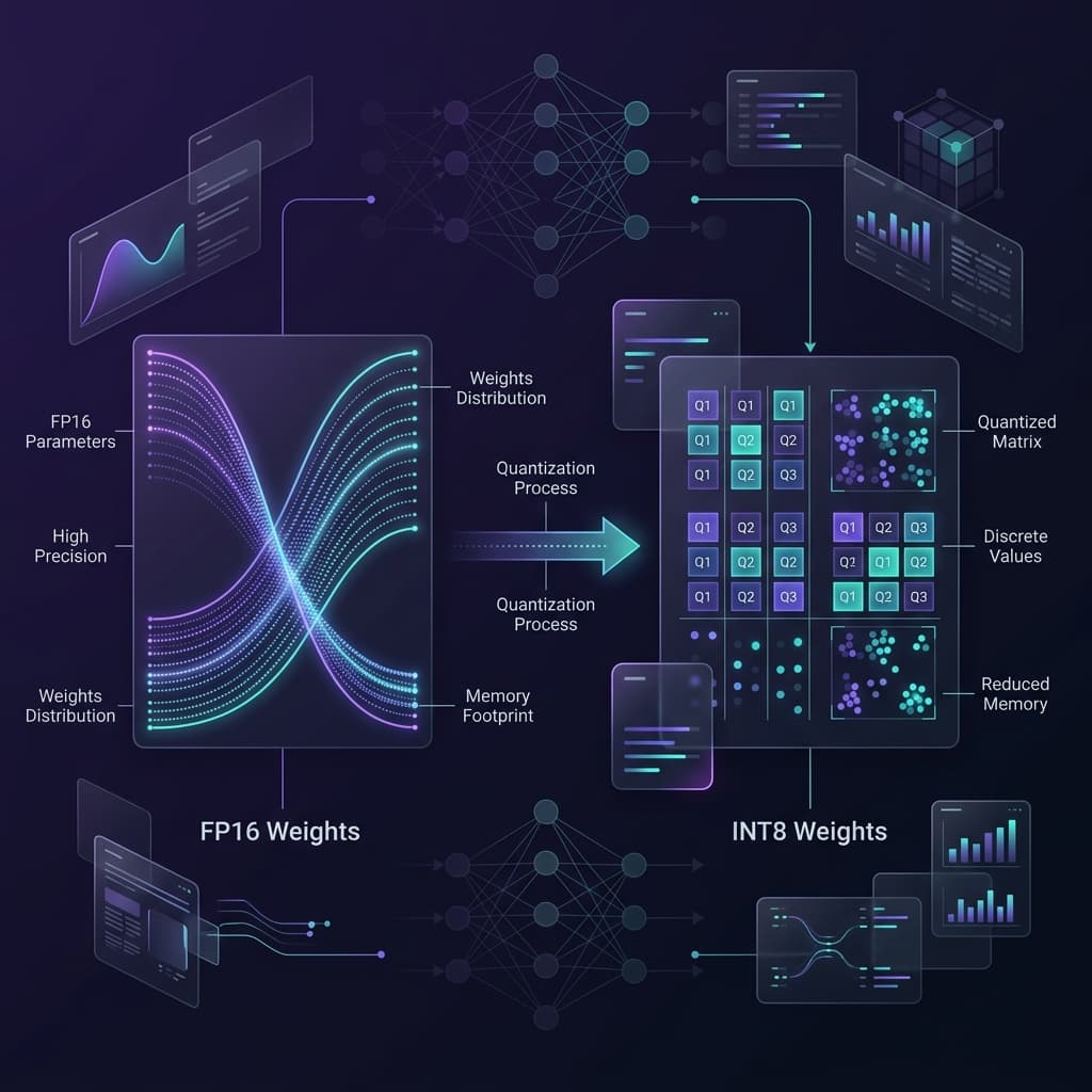
Quantization is the process of mapping continuous or high-precision floating-point numbers to lower-precision, discrete representations. In LLM optimization, quantization typically compresses 16-bit floating-point weights (FP16 or BF16) into 8-bit, 4-bit, or even 2-bit integers (INT8, INT4, INT2) or floating-point formats (FP8, FP4).
+-----------------------------------------------------------------------------------+
|                              QUANTIZATION LANDSCAPE                               |
+----------------------------------+------------------------------------------------+
|  POST-TRAINING QUANTIZATION (PTQ) |  QUANTIZATION-AWARE TRAINING (QAT)             |
|  - Performed after training      |  - Integrates quantization into training loop  |
|  - Requires hours of compute     |  - Requires massive compute and dataset access |
|  - Uses calibration dataset      |  - Retains higher accuracy at ultra-low bits   |
+----------------------------------+------------------------------------------------+
Post-Training Quantization (PTQ) is highly favored in enterprise environments because it operates on pre-trained models without requiring expensive retraining pipelines. Within the PTQ domain, the three leading methodologies serve distinct roles:
1. GPTQ (Generative Pre-trained Transformer Quantization)
GPTQ is a second-order, Hessian-guided post-training quantization algorithm. It operates on a "one-shot" basis, quantizing weights layer by layer using a calibration dataset. GPTQ minimizes the reconstruction error between the output of the original high-precision layer and the quantized layer by adjusting the remaining unquantized weights to compensate for the rounding error of already quantized weights.
2. AWQ (Activation-aware Weight Quantization)
AWQ is an activation-aware quantization methodology that does not rely on second-order error corrections. Instead, it operates on the observation that weight importance is not uniform; a small percentage (roughly 1%) of weights—called "salient weights"—dictate most of the model's accuracy. AWQ identifies these weights by observing activation distributions, and scales them up before quantization to protect them from rounding errors.
3. GGUF (formerly GGML)
GGUF is a unified file format and quantization framework built for the llama.cpp ecosystem. Rather than optimizing exclusively for GPU serving, GGUF is designed for hybrid CPU/GPU inference, Apple Silicon Unified Memory, and cross-platform portability. It uses hierarchical block-based quantization (K-quants) and mixed-precision layer configurations to optimize inference on consumer hardware.
The following table compares the high-level attributes of these three formats:
| Dimension | GPTQ | AWQ | GGUF |
|---|---|---|---|
| Core Optimization | Hessian-guided weight adjustment | Activation-aware salient weight scaling | Hierarchical block-wise mixed-precision |
| Calibration Requirement | Mandatory (typically 128 samples) | Mandatory (typically 32-128 samples) | Optional (for static K-quants) |
| Primary Target Hardware | NVIDIA GPUs | NVIDIA/AMD GPUs | CPU, Apple Silicon, Hybrid CPU/GPU |
| Primary Serving Engine | vLLM, TensorRT-LLM, AutoGPTQ | vLLM, TGI, SGLang, AutoAWQ | Ollama, llama.cpp, Llamafile |
| File Architecture | Separate weights + metadata | Separate weights + metadata | Single unified binary (.gguf) |
⚡ Why It Matters
To understand the engineering necessity of quantization, we must analyze the hardware limits of memory capacity and memory bandwidth.
The Memory Capacity Constraint
The raw size of a model's weights determines the minimum VRAM required to host the model. If a model cannot fit into the memory of a single GPU, it must be partitioned across multiple GPUs using Tensor Parallelism (TP) or Pipeline Parallelism (PP). This introduces inter-GPU communication latency over NVLink or PCIe, which degrades throughput.
Model Size (GB) = Parameter Count (Billions) * Bytes Per Parameter
For a 70-billion parameter model (like Llama 3 70B):
- At FP16 precision (2 bytes/param):
70 * 2 = 140 GB(Requires at least two 80GB GPUs). - At INT8 precision (1 byte/param):
70 * 1 = 70 GB(Fits on a single 80GB GPU). - At INT4 precision (0.5 bytes/param):
70 * 0.5 = 35 GB(Fits on a single 40GB or 48GB GPU).
By compressing the weights to 4-bit, we achieve a 4x reduction in required VRAM, enabling engineers to serve massive models on consumer-grade or mid-tier enterprise hardware (like NVIDIA L4 or A10G GPUs) instead of multi-GPU H100 nodes.
The Memory Bandwidth Bottleneck
During the autoregressive decoding phase, the batch size is often small (e.g., serving a single user or a small group of users). In this regime, the system is memory-bandwidth bound. For each generated token, the GPU must stream billions of weight parameters from High Bandwidth Memory (HBM) into its local registers (SRAM) to compute the attention weights.
If we serve Llama 3 8B at FP16 on a GPU with 1.5 TB/s memory bandwidth (such as an A10G):
- To load 16 GB of weights for one token generation step takes:
16 GB / 1.5 TB/s = 10.6 milliseconds. - This limits the maximum single-user generation speed to roughly 94 tokens per second, even if the compute cores run instantaneously.
If the model is quantized to 4-bit (reducing weight size to 4 GB):
- To load 4 GB of weights takes:
4 GB / 1.5 TB/s = 2.6 milliseconds. - This increases the upper limit of single-user generation speed to roughly 384 tokens per second.
Quantization directly addresses the memory wall. By streaming compressed weights and unpacking them on-the-fly inside the GPU SRAM, we reduce the volume of data transferred across the memory bus, yielding near-proportional increases in inference speed during memory-bound decoding.
🛠️ How It Works
Quantization maps a high-precision continuous value space to a lower-precision discrete value space. To understand the advanced algorithms of GPTQ and AWQ, we must first master basic linear uniform quantization.
Uniform Quantization Mathematics
Linear uniform quantization maps floating-point numbers to integers using a scale factor S and a zero-point Z. The scale factor is a positive floating-point number that defines the step size of the quantization bins, and the zero-point is an integer that maps the real value 0 to the quantized space.
For a real value x, the quantization formula is:
Q(x) = clamp(round(x / S) + Z, q_min, q_max)
Where:
q_minandq_maxrepresent the boundaries of the target integer format (e.g., -128 and 127 for signed INT8, or 0 and 15 for unsigned INT4).clamp(v, min, max)restricts the valuevto the range[min, max].
To recover the approximate real value during inference, we dequantize the integer representation:
Dequant(q) = S * (q - Z)
The scale S and zero-point Z are calculated based on the range of the input values [min_val, max_val]:
S = (max_val - min_val) / (q_max - q_min)
Z = round(( -min_val / S ) + q_min)
Asymmetric Quantization:
Real Space:      min_val <------------------- 0 -------------------> max_val
Quantized Space: q_min   <----------------- Z -------------------> q_max
(Zero-point Z is explicitly computed to align real 0)

Symmetric Quantization:
Real Space:     -max_abs <------------------- 0 -------------------> max_abs
Quantized Space: q_min   <------------------- 0 -------------------> q_max
(Zero-point Z is fixed to 0, restricting real 0 to quantized 0. Requires max_abs = max(|min_val|, |max_val|))
- Asymmetric Quantization uses the full range of the target integer format by explicitly computing
Z. This is useful for asymmetric weight distributions but adds register overhead during dequantization arithmetic. - Symmetric Quantization forces
Z = 0. The scale is computed usingS = max(|min_val|, |max_val|) / q_max. This simplifies the dequantization formula toDequant(q) = S * q, reducing dequantization instruction overhead in CUDA kernels, but wastes one quantization bin (e.g., representing -128 in INT8) to maintain symmetry.
Block-wise Quantization
In large language models, weight values are not uniformly distributed across the entire weight matrix. Often, a single layer matrix contains local clusters of highly varied weights. If we compute a single scale factor S for an entire matrix (per-tensor quantization), a single large outlier value forces S to be very large. This crushes the resolution of smaller, highly sensitive weights into a few quantization bins, resulting in severe accuracy loss.
To resolve this, modern quantization uses Block-wise (or Group-wise) Quantization. The weight matrix is partitioned into smaller contiguous blocks of size group_size (typically 32, 64, or 128 elements). A unique scale factor S and zero-point Z are calculated and stored for each individual group.
While a smaller group size improves accuracy by isolating outliers, it increases the memory overhead because more scale and zero-point parameters must be stored alongside the quantized weights. The table below illustrates this metadata overhead for 4-bit weights at FP16 scale precision:
| Group Size | Weights Size (Bits) | Scales Overhead (Bits/Weight) | Total Bits Per Weight | Metadata VRAM Overhead |
|---|---|---|---|---|
| Per-Tensor | 4.00 | < 0.01 | ~4.00 | Negligible |
| 128 | 4.00 | 16 / 128 = 0.125 | 4.125 | ~3.1% |
| 64 | 4.00 | 16 / 64 = 0.250 | 4.250 | ~6.2% |
| 32 | 4.00 | 16 / 32 = 0.500 | 4.500 | ~12.5% |
2. Architecture
GPTQ: Hessian-Guided Error Minimization
GPTQ is based on the framework of Optimal Brain Quantization (OBQ). Its objective is to find a quantized weight matrix W_hat that minimizes the squared reconstruction error of the layer outputs over a calibration dataset X:
argmin_W_hat || W * X - W_hat * X ||_2^2
Instead of quantizing each weight element independently using Round-to-Nearest (RTN), GPTQ treats quantization as a sequential optimization problem. It quantizes weights column-by-column and updates the remaining unquantized weights to compensate for the rounding error.
The mathematical formulation uses a second-order Taylor series expansion of the reconstruction error. The Hessian matrix of the squared error is:
H = 2 * X * X^T
Where X is the matrix of layer inputs from the calibration dataset. When quantizing the weight vector w_q at column q, the optimal adjustment delta w_q to apply to the remaining unquantized columns is:
delta w_q = - ( (w_q - quant(w_q)) / [H^-1]_qq ) * [H^-1]_:,q
Where:
w_q - quant(w_q)is the quantization error introduced by rounding the current column.[H^-1]_qqis theq-th diagonal element of the inverse Hessian matrix.[H^-1]_:,qis theq-th column of the inverse Hessian matrix.
After updating the current column to its quantized representation, the remaining unquantized columns (columns index > q) are adjusted:
W_:, >q = W_:, >q - delta w_q * H^-1_q, >q
To run this algorithm stably on massive weight matrices (such as Llama 3 70B layers of size 8192 x 28672), GPTQ employs a Cholesky decomposition of the inverse Hessian matrix:
H^-1 = L * L^T
Where L is a lower triangular matrix. The algorithm processes the weights in blocks (typically 128 columns at a time). It computes Cholesky factors for the block, applies the updates locally within fast GPU cache memory, and then propagates the updates to the rest of the matrix. This reduces the computational complexity of the second-order adjustments and prevents numerical instability.
Activation Order (act-order)
To improve quality, GPTQ can be configured with the act-order (or descending-order) heuristic. This heuristic sorts the columns of the weight matrix by the variance of their input activations prior to quantization, ensuring that columns with the highest activation variance (the most sensitive weights) are quantized first.
While act-order significantly reduces perplexity degradation on 3-bit and 4-bit models, it introduces a runtime performance penalty. Because sorting columns shuffles the physical weight layout, the GPU cannot perform coalesced memory access during dequantization. In early implementations, this resulted in a 30% to 50% drop in throughput. Modern GPU serving engines bypass this by integrating specialized kernels (like Marlin) that compile a lookup table to resolve memory layouts on-the-fly inside SRAM registers.
AWQ: Activation-Aware Salient Weight Protection
AWQ was designed to address the complexity and hardware inefficiency of GPTQ's second-order weight updates. The creators of AWQ observed that post-training quantization loss is dominated by a tiny fraction (1% or less) of the weights. These weights, termed "salient weights," correspond to the channels that process the largest input activation values.
In transformer architectures, LLM activations display a highly skewed distribution: a small number of hidden dimensions consistently have values that are orders of magnitude larger than the average. If these channels are quantized alongside normal channels, the large dynamic range of the outliers forces the scale factor S to be large, which destroys the precision of the remaining channels.
AWQ protects these salient channels without executing complex Cholesky updates. Instead, it applies a mathematically equivalent scaling factor S to the weights and activations prior to quantization:
Y = W * X = (W * diag(S)) * (diag(S)^-1 * X)
Where diag(S) is a diagonal matrix of channel-wise scaling factors S > 1. By scaling the weight columns W up by S, the salient weights are physically pushed into larger quantization bins, protecting them from rounding errors. The input activation channels X are scaled down by 1/S to maintain exact mathematical equivalence of the linear layer output Y.
To find the optimal scaling factors, AWQ parameterizes S as a function of the average input activation magnitude s_X:
S = s_X^alpha
Where s_X is the channel-wise average activation magnitude computed over a calibration dataset, and alpha is a scaling exponent in the range [0, 1]. The optimal alpha is determined via a grid search that minimizes the reconstruction error:
argmin_alpha Loss( quant(W * diag(s_X^alpha)) * diag(s_X^-alpha) * X - W * X )
AWQ Optimization Workflow:
1. Pass calibration data -> Compute average activation magnitude per channel (s_X).
2. Define search space for alpha (typically [0, 0.1, 0.2, ... 1.0]).
3. Loop alpha:
   a. Compute scaling factor S = s_X^alpha
   b. Scale weights: W_scaled = W * S
   c. Scale activations: X_scaled = X / S
   d. Quantize W_scaled to target bit-width.
   e. Compute reconstruction loss: || quant(W_scaled) * X_scaled - W * X ||
4. Select alpha that minimizes loss -> Apply scaling permanently to model weights.
Because this scaling is applied as a static pre-processing step, the inference engine does not need to execute scale calculations at runtime. The scaled weights are quantized and saved to disk. During inference, the engine simply loads the quantized weights and dequantizes them using the static scales, completely avoiding the memory shuffling and de-coalescing issues associated with GPTQ's act-order heuristic.
GGUF: Mixed-Precision K-Quants and Apple Silicon Optimization
GGUF is a successor to the GGML format, developed by Georgi Gerganov and the llama.cpp open-source community. Unlike GPTQ and AWQ, which focus on maximizing raw GPU throughput, GGUF is designed to run large models on heterogeneous consumer hardware (e.g., Apple M-series chips with unified memory, standard CPUs with RAM, and consumer-grade GPUs).
GGUF's design centers on three architectural pillars:
1. Single-File Layout and Memory-Mapped I/O
A GGUF file is a single binary file that contains both model metadata (such as vocabulary, tokenizer settings, layer dimensions, and hyperparameters) and the model weight tensors. The weights are aligned to specific byte boundaries, allowing the inference engine to use the mmap (memory map) system call. This maps the model file directly into the process's virtual address space, enabling near-instant startup times and allowing the operating system to manage memory caching dynamically.
2. Hierarchical Super-Block Structure (K-Quants)
GGUF utilizes "K-quants" (Kawrakow quantization), which employ a hierarchical super-block structure to minimize the storage overhead of quantization scale factors:
- A super-block contains 256 weights.
- This super-block is subdivided into 8 smaller blocks, each containing 32 weights.
- Each sub-block of 32 weights is quantized to the target bit-width (e.g., 4-bit).
- Instead of storing 16-bit float scale factors for every sub-block, K-quants use double quantization: the sub-block scales are quantized into 6-bit or 4-bit integers. A single 16-bit float scale is then stored for the entire 256-weight super-block to dequantize the sub-block scales.
This hierarchical compression reduces the metadata memory footprint of 4-bit quantization from 12% to less than 4%, preserving precious memory bandwidth on CPUs and unified memory buses.
3. Mixed-Precision Layer Configurations
GGUF supports mixed-precision quantization presets. Because different layers in a transformer architecture have different sensitivities to quantization noise, GGUF allocates higher bit-widths to critical layers while compressing less sensitive layers. For example, the Q4_K_M (medium) preset uses the following mixed structure:
- Attention
vandwolayers: Quantized to 4-bit (K-quants super-blocks). - Feed-Forward Network (FFN)
w2(down-projection) andw3(gate-projection) layers: Quantized to 6-bit. These layers represent the majority of the model's factual capacity and are highly sensitive to quantization errors. - Embeddings and Output Head: Quantized to 6-bit.
- Remaining Attention layers: Quantized to 4-bit.
This mixed-precision approach yields a model with an average bit-width of roughly 4.5 bits per weight, retaining near-FP16 perplexity while running efficiently in low-memory environments.
The table below provides a detailed structural comparison of the primary quantization formats:
| Property | GPTQ | AWQ | GGUF (K-Quants) |
|---|---|---|---|
| Quantization Scheme | Per-group (32, 64, 128) | Per-group (32, 64, 128) | Super-blocks (256) with sub-blocks (32) |
| Metadata Storage | 16-bit scales + zero-points | 16-bit scales + zero-points | Double-quantized scales (4/6-bit) + 16-bit super-scales |
| Model Structuring | Uniform bit-width per layer | Uniform bit-width per layer | Mixed-precision presets (Q4_K_M, Q5_K_M) |
| Memory Access | Non-coalesced if act-order is active | Fully coalesced | Fully coalesced via mmap |
| Supported Kernels | AutoGPTQ, ExLlamaV2, Marlin | AutoAWQ, vLLM, Marlin | llama.cpp custom SIMD/Neon/AVX2 kernels |
| Distributed Scaling | Native (Tensor Parallelism) | Native (Tensor Parallelism) | Limited (Single-node CPU/GPU offload) |
📊 Benchmarks
To evaluate the real-world impact of these quantization techniques, we compare the WikiText-2 perplexity, memory usage, and inference speed of Llama 3 8B.
WikiText-2 perplexity measures the model's ability to predict text sequences, where a lower perplexity indicates better retention of the model's reasoning capabilities. Speed is evaluated in tokens per second during the decoding phase.
- Hardware Platform: Single NVIDIA RTX 4090 GPU (24GB VRAM) for GPU formats; Mac Studio M3 Max (64GB Unified Memory) for GGUF.
- Context Length: 4096 tokens.
- Batch Size: 1 (Single-user stream).
The benchmark results are consolidated in the table below:
| Format / Preset | Bit-Width | VRAM / Memory (GB) | WikiText-2 Perplexity | Decode Speed (Tokens/sec) | Downstream Reasoning Retention |
|---|---|---|---|---|---|
| FP16 (Unquantized) | 16.00 | 16.00 | 6.23 | 55.4 | 100.0% (Baseline) |
| GGUF Q8_0 | 8.50 | 8.90 | 6.24 | 72.1 | 99.8% |
| GGUF Q5_K_M | 5.50 | 6.10 | 6.28 | 98.4 | 99.1% |
| GGUF Q4_K_M | 4.80 | 5.30 | 6.38 | 114.2 | 98.2% |
| AWQ INT4 (Group 128) | 4.12 | 4.60 | 6.30 | 148.6 | 98.7% |
| GPTQ INT4 (Group 128) | 4.12 | 4.60 | 6.33 | 152.3 (ExLlamaV2) | 98.5% |
| GPTQ INT4 + Marlin | 4.12 | 4.60 | 6.33 | 178.4 | 98.5% |
| GGUF Q3_K_M | 3.80 | 4.30 | 6.55 | 128.5 | 94.2% |
Key Benchmark Observations
- The Accuracy-Size Sweet Spot: Compressing from FP16 to 5-bit (
GGUF Q5_K_M) or 4-bit (AWQ INT4) yields a massive~70%reduction in memory consumption while increasing perplexity by only< 0.15points. This negligible precision loss has no observable impact on downstream tasks like chat, classification, or summarization. - GPTQ vs. AWQ Performance: AWQ achieves slightly lower perplexity than GPTQ because its activation-aware scaling protects salient weights. However, GPTQ (using the ExLlamaV2 kernel) exhibits a minor speed advantage due to highly optimized layout configurations.
- The Marlin Acceleration: Integrating the Marlin kernel with GPTQ models boosts decode speed to 178.4 tokens/second. Marlin achieves this by scheduling FP16-INT4 GEMM operations inside the GPU register file, minimizing the overhead of on-the-fly weight unpacking.
- GGUF Speed on Apple Silicon: On Apple Silicon M3 Max,
GGUF Q4_K_Machieves 114.2 tokens/second. The unified memory architecture allows the Apple GPU to access the model weights directly without transferring data over a PCIe bus, providing server-grade performance in a local workstation environment.
⚙️ Production Deployment Considerations
Deploying quantized models in high-concurrency enterprise environments requires analyzing how different formats scale across hardware architectures.
Distributed Scaling: Tensor Parallelism vs. Pipeline Parallelism
When serving large models (such as Llama 3 70B), a single GPU may not have enough VRAM to host both the model and the KV cache. To scale the model, we partition the layer matrices across multiple GPUs.
+-----------------------------------------------------------------------------------+
|                            DISTRIBUTED SERVING ENGINES                            |
+------------------------------------+----------------------------------------------+
|  TENSOR PARALLELISM (TP)           |  PIPELINE PARALLELISM (PP)                   |
|  - Partitions weight matrices      |  - Splits model layers sequentially          |
|    column-wise/row-wise.           |    across multiple GPUs.                     |
|  - All GPUs execute concurrently.  |  - Introduces GPU idle time                  |
|  - Requires low-latency NVLink.    |    (pipeline bubbles).                       |
+------------------------------------+----------------------------------------------+
How quantization formats interact with distributed serving:
- GGUF does not natively support multi-node Tensor Parallelism. It is restricted to single-node deployments where it uses CPU thread offloading and single-node multi-GPU layer splitting (Pipeline Parallelism). This makes GGUF unsuitable for high-throughput enterprise APIs.
- GPTQ and AWQ are natively supported by distributed serving engines like
vLLMandTensorRT-LLM. The weights are stored as packed integers. During inference, the engine performs Tensor Parallelism calculations by launching CUDA kernels that split the packed weights across NVLink connections. - Hopper Native FP8: For deployments using NVIDIA H100, H200, or Blackwell GPUs, FP8 (8-bit floating-point) has become the industry standard. Hopper architectures feature native FP8 Tensor Cores that execute FP8 matrix multiplication directly. This eliminates the need to unpack weights to FP16, bypassing the dequantization penalty entirely while maintaining near-perfect FP16 perplexity.
Specialized Dequantization Kernels
To optimize inference speed, serving engines utilize specialized CUDA kernels that minimize register pressure during weight unpacking:
- Marlin: A highly optimized FP16-INT4 matrix multiplication kernel. Marlin is designed for low-batch decoding, where memory bandwidth is the primary constraint. It uses a structured thread-mapping layout to load quantized weights into shared GPU memory and unpack them in registers, achieving near-theoretical peak HBM bandwidth utilization.
- ExLlamaV2 (EXL2): A custom format and kernel suite popular in the local GPU community. EXL2 supports variable-bit quantization, allowing different layers within the same model to be quantized to different bit-widths (e.g., mixing 3-bit, 4-bit, and 5-bit layers). This allows users to fit a model precisely within a specific VRAM budget (like 16GB or 24GB).
❌ Common Mistakes
Deploying quantized models in production often exposes subtle failure modes. Below are the most common mistakes made by infrastructure engineers:
1. Mismatched Calibration Datasets
GPTQ and AWQ rely on a calibration dataset to determine weight saliency and execute second-order updates. If a model is quantized using a generic English dataset (such as the Pile) but deployed for specialized domains (such as coding or biomedical translation), it will experience catastrophic accuracy loss.
For instance, calibrating a code-generation model with standard conversational text will crush the precision of weights that process syntax structures like curly braces and brackets. Always use a calibration dataset that matches the target deployment domain.
2. Using act-order in GPTQ without Marlin Integration
Enabling the act-order heuristic in GPTQ improves perplexity by quantizing sensitive columns first, but it shuffles the weight layout. If deployed on standard serving frameworks without specialized kernels, the GPU cannot coalesce memory reads. This turns a memory-bandwidth-bound operation into a latency disaster, reducing decoding speed by up to 50%.
If you enable act-order, you must ensure that your serving engine utilizes the Marlin kernel or ExLlamaV2 to handle the physical memory mapping.
3. Neglecting the Dequantization Penalty at High Batch Sizes
Quantization is highly effective at small batch sizes because the workload is memory-bandwidth bound. However, as the batch size increases (e.g., batch_size > 32), the workload becomes compute-bound.
Because standard GPUs cannot perform INT4 matrix multiplications directly, the dequantization kernels must unpack the INT4 weights back to FP16 in local SRAM registers before executing the Tensor Core operations. At high batch sizes, the time spent performing this unpacking (the dequantization penalty) can exceed the memory savings, resulting in lower total throughput compared to native FP16 or FP8 execution.
Low Batch Size (Memory-Bound):
[Read INT4 Weights (Small size)] --(Fast Transfer)--> [SRAM] --(Dequant to FP16)--> [Compute]
==> Latency is reduced because transfer time dominates.

High Batch Size (Compute-Bound):
[Read INT4 Weights (Small size)] --(Transfer)--> [SRAM] --(Dequant overhead dominates)--> [Compute]
==> Throughput degrades due to constant unpacking register pressure.
📈 Lessons From Production Deployments
Operating large-scale LLM endpoints reveals several key lessons regarding model compression and memory management:
1. The Context-Weight VRAM Balance
In long-context applications (e.g., serving 128k context windows), the memory footprint of the Key-Value (KV) cache can quickly surpass the size of the model weights. For example, serving Llama 3 8B at FP16 with a 128k context requires:
KV Cache Size = 2 * 1 * 131072 * 8 * 128 * 2 = 536,870,912 bytes ≈ 536 MB (Per active user)
At a batch size of 32, the KV cache requires 17.1 GB of VRAM, while the model weights require only 16 GB. In this regime, compressing model weights to 4-bit saves only 12 GB, which is quickly consumed if KV cache allocation is not optimized.
To achieve maximum concurrency, weight quantization must be paired with KV cache quantization (such as FP8 or INT8 KV cache) and page block optimization via PagedAttention.
2. Memory Fragmentation and gpu_memory_utilization in vLLM
When deploying AWQ or GPTQ models on vLLM, the engine pre-allocates a chunk of VRAM for the KV cache pool based on the gpu_memory_utilization configuration parameter. If this parameter is set too high (e.g., 0.95), the engine may not leave enough free VRAM for the dequantization kernels to load temporary variables. This results in runtime out-of-memory (OOM) errors during peak concurrency.
Production environments should set gpu_memory_utilization to 0.85 or 0.90 to provide a safety buffer for kernel execution.
3. Latency vs. Throughput Trade-offs
When designing an LLM serving pipeline, engineers must choose between optimizing for time-to-first-token (TTFT) or throughput (tokens/second/system):
- For TTFT-sensitive applications (like real-time agents), native FP16 or FP8 models are preferred. The prefill phase is compute-bound, and avoiding dequantization unpacking reduces the initial response latency.
- For throughput-sensitive applications (like batch document processing), 4-bit AWQ or GPTQ models are superior. They allow for larger batch sizes, which maximizes the total volume of text processed per GPU hour.
🔍 What Most Articles Miss
Many general overviews of LLM quantization omit the underlying mathematical reasons for why activation outliers occur and how dequantization interacts with GPU registers.
The Mathematics of Outlier Activations
To understand why AWQ's channel-wise scaling is mathematically superior to standard Round-to-Nearest quantization, we must examine why activation outliers emerge.
In transformer models with more than 6.7 billion parameters, a phenomenon occurs where a tiny fraction of hidden dimensions (typically < 0.1% of channels) develop extremely large values (e.g., 100x larger than average). These outliers are not random noise; they emerge during training as coordinate anchors that the model uses to track syntax state and long-context associations.
Standard Quantization (No scaling):
Channel 1 (Normal):  [-0.2, 0.5, 0.1]  ==> Scales to fit outlier range ==> Rounding error crushes precision
Channel 2 (Outlier): [0.1, 128.0, 0.2] ==> Dictates the scale factor S

AWQ Scaling (diag(S)):
W_new = W * S,  X_new = X / S
(Outliers in X are scaled down, normal values are protected in W by scaling up.
The dynamic range of the entire tensor is balanced, preserving resolution across all channels.)
Standard uniform quantization computes the scale factor S based on the maximum value in the tensor. When an outlier of 128.0 is grouped with normal values of 0.2, the resulting scale factor is so large that the normal values are rounded to zero, destroying the model's capacity to represent subtle semantic relationships.
AWQ's diagonal scaling matrix diag(S) resolves this. By scaling the outlier activation channels down by 1/S, we compress their dynamic range. To maintain mathematical equivalence, the corresponding weight columns are scaled up by S.
When quantization is applied, the weights corresponding to the outlier channels are protected from rounding error by their larger physical values, while the weights for the normal channels are quantized using a smaller, higher-resolution scale factor. This preserves the representation capacity of both normal and outlier channels.
The GPU Register Pressure Bottleneck
A common misconception is that running a 4-bit model reduces GPU thermal load. In reality, dequantizing INT4 weights on-the-fly to FP16 during decoding increases GPU register pressure.
During a matrix-vector multiplication (GEMV), the GPU threads must:
- Load the packed 4-bit integers from VRAM.
- Unpack the 4-bit integers into individual 16-bit float registers.
- Apply the scale factor and zero-point.
- Perform the multiply-accumulate operation on the FP16 Tensor Cores.
This unpacking process requires bit-shifting and masking operations that run on the GPU's integer ALUs, consuming registers that would otherwise be used to store input activations or KV cache pointers.
If the model size is large, this register pressure can lead to instruction stalls. This explains why FP8 is highly favored on modern Hopper GPUs: because the hardware supports FP8 tensor arithmetic natively, the weights are streamed and computed without requiring integer unpacking, bypassing the register bottleneck entirely.
💡 Best Practices
When deploying quantized models in production, follow these guidelines to optimize the balance between accuracy, memory footprint, and speed:
- Workstation and Local Deployment: Use GGUF format with the
Q4_K_MorQ5_K_Mpresets. This configuration balances CPU/GPU offloading and minimizes startup time viammap. - Enterprise GPU Serving (Hopper/Blackwell): Use FP8 (E4M3 format for weights) via
vLLMorTensorRT-LLM. This configuration avoids dequantization overhead by utilizing native FP8 Tensor Cores, providing near-FP16 accuracy with INT8-level memory savings. - Enterprise GPU Serving (Ampere/Ada Lovelace): Use 4-bit AWQ with a group size of 128. Ampere GPUs (like the A100 or A10G) lack native FP8 arithmetic support, making AWQ the optimal format for maximizing memory bandwidth efficiency.
- Low-Batch Latency Optimization: If serving single-user real-time streams (low latency), deploy GPTQ or AWQ models with the Marlin kernel enabled in vLLM. Marlin minimizes the register pressure of dequantization unpacking.
- Domain Calibration: If a model has been fine-tuned for a specific domain (such as SQL generation or legal analysis), do not use pre-quantized models from Hugging Face. Quantize the model yourself using a calibration dataset representative of the target domain.
- KV Cache Optimization: For long-context models (context window
> 32k), always pair weight quantization with FP8 KV cache quantization. This prevents the KV cache from consuming the VRAM saved by compressing the model weights.
❓ FAQ
1. What is the main difference between GPTQ and AWQ?
GPTQ uses second-order Hessian-guided optimization to update the remaining unquantized weights column-by-column to compensate for quantization errors. AWQ does not alter weights to minimize error; instead, it observes activation distributions, identifies the most important 1% of channels, and scales them up before applying simple rounding quantization to protect them from precision loss.
2. Can I run GGUF models on a GPU?
Yes. GGUF engines (such as llama.cpp and Ollama) support GPU offloading. You can specify the number of layers to offload to the GPU's VRAM, while the remaining layers run on the CPU. If you have enough VRAM to fit the entire GGUF model, it can run entirely on the GPU, though its execution speed may be slightly slower than formats like AWQ or GPTQ.
3. Why does quantization increase perplexity?
Quantization maps continuous real numbers to a discrete set of integers. This rounding process discards high-frequency information, introducing quantization noise. This noise degrades the model's precision, resulting in a minor increase in perplexity.
4. Is FP8 quantization better than INT4?
Yes, in terms of accuracy. FP8 retains near-FP16 perplexity and is supported natively by newer GPU architectures (like Hopper and Blackwell), eliminating dequantization overhead. However, INT4 offers greater memory savings (compressing models by 4x compared to FP16, whereas FP8 compresses them by 2x).
5. What is the dequantization penalty?
The dequantization penalty is the processing overhead introduced by unpacking low-bit weights (like INT4) back into high-precision formats (like FP16/BF16) inside the GPU's SRAM registers before they can be executed on Tensor Cores. At high batch sizes, this unpacking process can become a bottleneck.
6. Can I fine-tune a quantized model?
Standard quantized formats (such as GPTQ, AWQ, and GGUF) are read-only and cannot be fine-tuned directly because integer weights lack the continuous gradient representations required for backpropagation. However, you can fine-tune them using Parameter-Efficient Fine-Tuning (PEFT) methods like QLoRA, which freeze the quantized base weights and train high-precision adapter matrices (FP16/BF16) on top of them.
7. Does GGUF support Tensor Parallelism?
GGUF does not support native multi-node Tensor Parallelism (splitting matrix multiplications across GPUs over NVLink). It supports Pipeline Parallelism (assigning sequential layers to different GPUs), which is slower than Tensor Parallelism due to pipeline synchronization delays.
8. What is the impact of group size in quantization?
Group size defines the number of weight elements that share a single scale factor and zero-point. A smaller group size (e.g., 32) improves accuracy by isolating outlier values but increases the VRAM overhead of storing scale metadata. A larger group size (e.g., 128) reduces metadata overhead but can lead to higher perplexity.
9. Why is calibration data necessary for post-training quantization?
Calibration data is used to observe the model's activation distributions during inference. GPTQ uses this data to compute the Hessian matrix for error correction, and AWQ uses it to identify which channels exhibit the largest activation magnitudes (outliers) and require scaling.
10. Can I run a 70B model on a single 24GB GPU?
Yes. A 70B parameter model quantized to 2-bit or 3-bit GGUF/EXL2 can fit within 24GB of VRAM. However, models quantized to 2-bit or 3-bit often exhibit noticeable accuracy degradation and hallucination, making 4-bit the recommended minimum for reliable reasoning.
📌 Key Takeaways
- Memory Wall Resolution: Post-Training Quantization (PTQ) is essential for modern LLM deployment, compressing model weights by 4x (for INT4) to enable serving on commodity or single-GPU instances.
- Method Optimization Targets: GGUF is optimized for local consumer hardware and hybrid CPU/GPU architectures; AWQ is optimized for high-fidelity GPU serving; GPTQ is optimized for raw GPU throughput using dequantization kernels.
- Outlier Protection is Critical: AWQ prevents accuracy loss by identifying activation outliers and scaling those channels up before quantization, outperforming simple Round-to-Nearest approaches.
- Dequantization Penalty: Low-bit integer quantization (INT4/INT3) requires unpacking weights to FP16 during decoding, which can introduce computational bottlenecks at high batch sizes.
- Hopper and Blackwell FP8 Standards: FP8 has become the standard for enterprise GPU deployment on Hopper/Blackwell hardware, utilizing native FP8 Tensor Cores to bypass dequantization overhead entirely.
- KV Cache Scaling: For long-context workloads, weight quantization must be paired with PagedAttention and KV cache quantization (FP8/INT8) to prevent the KV cache from exceeding the model weight memory footprint.
