Scaling Embeddings: Vector Quantization (Scalar vs Binary Quantization)
How to reduce vector store memory footprints by 90% while maintaining semantic recall.

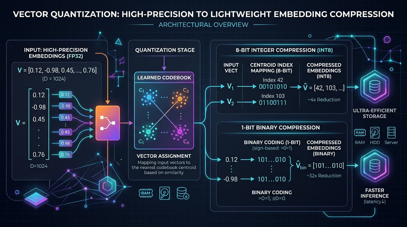
In the building of large-scale AI applications, the cost of scaling vector search infrastructure has become one of the most significant challenges for engineering teams. Modern transformer-based models output high-dimensional dense embeddings (for example, 1536 dimensions for OpenAI's text-embedding-3-small and 3072 dimensions for text-embedding-3-large). Storing these vectors in standard, uncompressed 32-bit floating-point formats (float32) quickly exhaust the memory capacity of production servers.
When a database holds millions of vectors, maintaining them entirely in random-access memory (RAM) is required to achieve sub-10ms query latencies. However, memory-optimized cloud instances are expensive. If a team is forced to scale their databases horizontally, hosting costs can grow from hundreds of dollars a month to tens of thousands. To understand the tradeoffs between specialized hardware and relational infrastructure, see our comprehensive analysis of Vector Databases in 2026: Pure Vector Stores vs PostgreSQL (pgvector) Extensions.
Vector Quantization (VQ) has emerged as the standard solution for scaling database memory footprint. By converting high-precision numbers into compressed representations, vector quantization reduces memory requirements by 75% to over 96%, while maintaining high retrieval accuracy. This architectural deep-dive examines the mathematics, implementation, database support, and production strategies for Scalar Quantization (SQ) and Binary Quantization (BQ).
What Is It?
Vector Quantization is a lossy compression technique that maps a high-dimensional vector space containing infinite possible floating-point combinations into a finite, discrete set of representations. In the context of vector databases, quantization does not compress the model itself; instead, it compresses the generated embeddings before they are written to the database index.
To understand the core differences, let us evaluate the two primary methods:
1. Scalar Quantization (SQ)
Scalar Quantization operates at the individual dimension level (scalar level). It maps a continuous range of 32-bit floating-point values (float32) to a discrete range of lower-precision numbers, typically 8-bit integers (int8 or uint8).
- Precision Reduction: Each dimension of a vector, which originally required 4 bytes of storage, is compressed into a single 1-byte representation.
- Compression Ratio: This yields a 4x reduction in total memory footprint.
- Distance Metrics: Similarity is computed using integer-arithmetic variants of Cosine or L2 Euclidean distance.
2. Binary Quantization (BQ)
Binary Quantization is an extreme form of compression. It reduces each dimension of a vector to a single bit, representing whether the floating-point value is positive or negative.
- Precision Reduction: Each dimension is binarized to a
0or1. A 1536-dimensional vector that requires 6144 bytes infloat32is compressed into a 1536-bit block, which takes only 192 bytes of storage. - Compression Ratio: This yields a 32x (or 96.8%) reduction in memory footprint.
- Distance Metrics: Similarity is calculated using Hamming distance, which measures the number of differing bits between two binary sequences.
3. Half-Precision Quantization (float16)
While not as aggressive as SQ or BQ, half-precision (float16 or halfvec in PostgreSQL) maps 32-bit floats to 16-bit floats. This provides a 2x memory reduction with virtually zero recall loss (typically less than 0.1% degradation). It serves as a safe first step before implementing more lossy compression schemes. To compare this with model weights quantization, check out our guide on Quantization Mathematics: GPTQ, AWQ, and GGUF Internals.
Here is a baseline comparison of these methods:
| Feature | Scalar Quantization (SQ8) | Binary Quantization (BQ) | Half-Precision (float16) |
|---|---|---|---|
| Data Type | int8 / uint8 | bit / binary | float16 / halfvec |
| Bytes per Dimension | 1 Byte | 0.125 Bytes (1 bit) | 2 Bytes |
| Memory Reduction | 4x (75% savings) | 32x (96.8% savings) | 2x (50% savings) |
| Distance Metric | Integer Cosine/Euclidean | Hamming / Jaccard | Cosine / Euclidean |
| Typical Recall Retention | 95% to 99% | 70% to 90% (Pre-Rerank) | 99.9% to 100% |
| Search Speed | 2x to 3x Faster | 10x to 40x Faster | 1.2x to 1.5x Faster |
| Best Use Case | Balanced precision & savings | Massive scale, fast pre-filtering | High-accuracy applications |
Why It Matters
The primary driver for vector quantization is database cost reduction and scalability. To illustrate this, let us calculate the physical memory requirements of a production vector database.
Suppose we need to store 10,000,000 vectors of 1536 dimensions. If we store these vectors in raw float32 representation:
Memory for Vectors = 10,000,000 * 1536 * 4 bytes = 61,440,000,000 bytes (approximately 57.22 GB)
However, a vector database does not just store the raw vectors; it must also build an index to enable fast similarity search. The standard index for production is the Hierarchical Navigable Small World (HNSW) graph. An HNSW graph maintains a multi-layer network of links between vectors. The memory overhead of these links depends on the parameters chosen (such as M, the number of bi-directional links per node). In production, HNSW graph links add between 50% and 100% memory overhead. For a detailed breakdown of graph construction, see Vector Indexing Under the Hood: HNSW vs IVF-PQ vs Flat Vector Indexes.
Thus, our 10 million vector database requires:
Total Memory (float32 HNSW) = Vector Storage (57.22 GB) + Index Overhead (~57.22 GB) = 114.44 GB of RAM
To support this dataset in-memory with safety overhead, we would need a cloud server instance with at least 128 GB or 256 GB of RAM, costing over $500 per month. If our dataset grows to 100 million vectors, we need over 1.1 TB of RAM, requiring a multi-node cluster costing thousands of dollars per month.
Now let us look at the memory requirements when using Scalar Quantization (int8):
Vector Storage (int8) = 10,000,000 * 1536 * 1 byte = 15,360,000,000 bytes (approximately 14.30 GB)
Index Overhead = ~14.30 GB
Total Memory (int8 HNSW) = 28.60 GB of RAM
Using Scalar Quantization reduces our RAM requirement to under 32 GB, allowing the entire database to run on a single inexpensive instance.
If we apply Binary Quantization:
Vector Storage (Binary) = 10,000,000 * 1536 * 0.125 bytes = 1,920,000,000 bytes (approximately 1.78 GB)
Index Overhead = ~1.78 GB
Total Memory (Binary HNSW) = 3.56 GB of RAM
With Binary Quantization, 10 million vectors can fit onto a lightweight server, reducing infrastructure costs by more than 95%. This enables teams to run local development databases and edge-node caching layers that would otherwise be impossible.
How It Works
Understanding how quantization compress values requires looking at the mathematical transformations and hardware-level operations that happen during indexing and retrieval.
+-------------------------------------------------------------+
|                     Vector Embedding                        |
|    [ 0.142, -0.891, 0.053, 0.412, -0.119, ... , 0.721 ]     |
+-------------------------------------------------------------+
                               |
            +------------------+------------------+
            |                                     |
            v                                     v
+------------------------+             +------------------------+
|  Scalar Quantization   |             |  Binary Quantization   |
|   (Scale & Translate)  |             |      (Sign Check)      |
|  Range: -128 to +127   |             |     Range: 0 or 1      |
+------------------------+             +------------------------+
            |                                     |
            v                                     v
+------------------------+             +------------------------+
|  [ 18, -114, 6, 52 ]   |             |   [ 1, 0, 1, 1, 0 ]    |
|       (1 Byte/Dim)     |             |      (1 Bit/Dim)       |
+------------------------+             +------------------------+
            |                                     |
            v                                     v
+------------------------+             +------------------------+
|  Integer Arithmetic    |             |  Hamming Distance      |
|  (AVX-512 SIMD Speedup) |             |  (XOR + Popcount CPU)  |
+------------------------+             +------------------------+
1. The Mathematics of Scalar Quantization
Scalar Quantization (specifically SQ8) projects floating-point values from a continuous range onto a fixed grid of 256 values. To do this, the database first scans a sample dataset of embeddings to find the minimum value (min_val) and maximum value (max_val) across all dimensions, or per dimension.
The transformation formula to convert a float32 dimension x into an 8-bit signed integer q is:
Quantized Value (q) = round(((x - min_val) / (max_val - min_val)) * 255) - 128
To reconstruct (dequantize) the value back to an approximate float x_approx during distance calculations, the inverse formula is applied:
Dequantized Value (x_approx) = min_val + ((q + 128) / 255) * (max_val - min_val)
Because finding the global minimum and maximum across the entire database can lead to skewed distributions due to outliers, modern vector databases often use Product Quantization (PQ) or Asymmetric Scalar Quantization, where the range is calculated per vector or per dimension block.
2. The Mathematics of Binary Quantization
Binary Quantization simplifies this process by focusing entirely on the sign of each float. The binarization function B(x) maps a float x to a single bit:
B(x) = 1 if x >= 0
B(x) = 0 if x < 0
During retrieval, instead of calculating the Cosine Similarity or Euclidean Distance using floating-point multiplication, we compare the binary vectors using Hamming Distance. The Hamming distance between two binary vectors is the number of positions at which the corresponding bits are different.
At the hardware level, this is implemented using a bitwise XOR followed by a population count (popcount) instruction, which counts the number of set bits (ones) in a CPU register.
Hamming Distance = Popcount(Vector_A XOR Vector_B)
Modern CPU architectures (such as AMD and Intel chips supporting AVX-512 or ARM processors supporting NEON) can execute XOR and popcount on registers containing hundreds of bits in a single CPU cycle. This makes binary vector search extremely fast compared to floating-point multiplication.
3. Statistical Binary Quantization (SBQ)
Standard Binary Quantization uses 0 as the split threshold. However, if the coordinates of our embeddings are not centered around zero, or if some dimensions have different variances, thresholding at zero results in severe information loss.
To solve this, Timescale developers introduced Statistical Binary Quantization (SBQ) in their pgvectorscale on GitHub extension. SBQ does not use a fixed zero threshold. Instead, it computes the statistical mean and variance of each dimension across a sample dataset. The binarization threshold for dimension i is set to its mean mean_i.
Furthermore, SBQ stores a small set of metadata alongside the binary vector (for example, the average magnitude of the vectors) to allow for asymmetric distance estimation, recovering a large portion of the lost recall.
4. Matryoshka Representation Learning (MRL)
To get the most out of quantization, we can pair it with Matryoshka Representation Learning (MRL). Developed by researchers at Google and academic institutions, MRL trains embedding models to store the most critical semantic information in the earliest dimensions of the vector.
For example, when using OpenAI's text-embedding-3-large, the model generates a 3072-dimensional vector. With MRL support, we can truncate this vector to 256 or 512 dimensions by simply discarding the trailing dimensions.
- Truncating a
float32vector from 3072d to 256d reduces its size by 12x. - If we then apply Binary Quantization to the remaining 256 dimensions, the vector is compressed to just 32 bytes (a 96x reduction from the original 12,288 bytes).
- Retrieval benchmarks show that this combination retains over 90% of the original search recall.
To understand how high-density chunk extraction and semantic parsing interact in retrieval pipelines, read our guide on Advanced RAG: Hierarchical Node Parsing, Parent-Child Retrievers, and Metadata Pre-Filtering.
Architecture
Implementing vector quantization depends heavily on the capabilities of the database engine you choose. Let us look at how quantization is handled in three major database environments.
+-----------------------------------------------------------------------+
|                       Quantization Implementations                    |
+-----------------------------------------------------------------------+
|  1. Qdrant (Rust-based)                                               |
|     - Native SQ (int8) & BQ (Hamming)                                 |
|     - 1.5-bit / 2-bit Quantization                                    |
|     - Automatic Asymmetric Rescoring / Reranking                      |
+-----------------------------------------------------------------------+
|  2. pgvector (Postgres C Extension)                                   |
|     - halfvec (float16) type reduces memory by 50%                     |
|     - bit(N) type for Binary Quantization                             |
|     - Native Hamming Distance: Vector_A <=> Vector_B                  |
+-----------------------------------------------------------------------+
|  3. pgvectorscale (Postgres Rust Extension)                           |
|     - StreamingDiskANN Index (Disk-resident vectors)                  |
|     - Statistical Binary Quantization (SBQ)                           |
+-----------------------------------------------------------------------+
1. Qdrant
Qdrant is a dedicated vector database written in Rust. It offers some of the most mature quantization controls in the industry.
- Native Scalar Quantization: Qdrant can automatically compress incoming
float32vectors toint8. The database maintains a small calibration dataset to determine the quantization ranges. - 1.5-bit and 2-bit Quantization: To bridge the gap between Scalar and Binary quantization, Qdrant supports 1.5-bit and 2-bit formats, which assign dimensions to three or four discrete states instead of two, saving memory while improving recall.
- Built-in Rescoring: Qdrant supports "oversampling and rescoring" directly in the query pipeline. The search is executed on the quantized HNSW index to find the top candidate matches (e.g.,
limit * 10). The database then retrieves the original, uncompressed vectors from disk and re-calculates the exact distance for those candidate matches, ensuring high recall.
2. pgvector (PostgreSQL Extension)
Starting with version 0.7.0 and continuing through version 0.8.x and pgvector v0.8.3 in 2026, pgvector has added native support for quantized indexes.
halfvecType:pgvectorintroduces thehalfvecdata type, which represents a 16-bit float. You can cast your vectors tohalfvecto save 50% of memory and disk space.- Binary Indexing with
bitType: Standard PostgreSQL supports a bit-string data type calledbit(N).pgvectorleverages this type for binary quantization. You can store your binarized vectors in abit(N)column and build an HNSW index using thebit_hamming_opsorbit_jaccard_opsoperator classes.
Here is an example of setting up a binary quantized table and HNSW index in PostgreSQL using pgvector:
-- Step 1: Create a table to store both the original float32 vector and the quantized bit vector
CREATE TABLE document_embeddings (
    id SERIAL PRIMARY KEY,
    content TEXT,
    -- Store the original float32 vector for re-ranking
    embedding vector(1536),
    -- Store the binarized vector for fast graph search
    embedding_binary bit(1536)
);

-- Step 2: Build an HNSW index on the binary representation using Hamming Distance
-- This index fits entirely in RAM because it is composed of bits
CREATE INDEX ON document_embeddings
USING hnsw (embedding_binary bit_hamming_ops)
WITH (m = 16, ef_construction = 64);
To insert data, we binarize the vector. If you are using standard float32 vectors, you can binarize them in your application layer (e.g., in Python or TypeScript) or use a helper function. Here is how you execute a two-step oversampled retrieval query in SQL:
-- Step 3: Execute search with binary indexing and float32 re-ranking
WITH candidate_documents AS (
    -- Subquery: Retrieve 100 candidate matches using fast binary Hamming distance
    SELECT
        id,
        content,
        embedding,
        (embedding_binary <=> '10110011...'::bit(1536)) AS hamming_distance
    FROM document_embeddings
    ORDER BY embedding_binary <=> '10110011...'::bit(1536)
    LIMIT 100
)
-- Main Query: Re-rank the 100 candidates using exact Cosine Distance on full float32 embeddings
SELECT
    id,
    content,
    (embedding <=> '[0.012, -0.045, ...]'::vector(1536)) AS exact_cosine_distance
FROM candidate_documents
ORDER BY exact_cosine_distance
LIMIT 10;
3. pgvectorscale (Timescale Rust Extension)
While pgvector provides the basic types, Timescale’s pgvectorscale extension optimizes this setup for enterprise-scale databases.
- StreamingDiskANN: Instead of holding all vectors in memory, StreamingDiskANN stores the compressed quantization index in memory, while writing the full-precision
float32vectors to disk. During search, the index identifies candidates, and the engine streams the raw vectors from disk to perform the final re-ranking. This avoids the RAM limits of PostgreSQL. - Native SBQ: It automates the Statistical Binary Quantization process directly inside the index build pipeline, saving developers from manually calculating dimension thresholds.
To see how these indexing styles fit into hybrid query layouts, read Hybrid Search: Reciprocal Rank Fusion (RRF) and Cross-Encoder Reranking.
Database Quantization Support Matrix
The following matrix compares quantization support across major vector database platforms in 2026:
| Database / Extension | Native SQ (int8) | Native BQ (bit / 1-bit) | Native PQ (Product) | Native float16 (halfvec) | Disk-Resident Vector Re-Ranking |
|---|---|---|---|---|---|
| Qdrant (v1.10.x) | Yes | Yes | Yes | Yes | Yes (Oversampling & Rescore) |
| pgvector (v0.8.x) | Yes (via cast) | Yes (via bit type) | No | Yes (via halfvec) | No (requires manual SQL CTEs) |
| pgvectorscale (v0.9.x) | Yes | Yes (via SBQ) | No | Yes | Yes (via StreamingDiskANN) |
| Milvus (v2.5.x) | Yes | Yes | Yes | Yes | Yes (DiskANN implementation) |
| Vespa.ai | Yes | Yes | Yes | Yes | Yes (Tensor-level HNSW) |
Embedding Model Quantization Suitability
Not all embedding models perform equally under quantization. Models trained with standard MSE or cosine loss functions will experience significant recall degradation when compressed to 1 bit per dimension.
In contrast, "quantization-aware" models are trained with regularizers that force dimension values to group around the extremes (-1 and +1 or similar), meaning little information is lost when binarizing.
| Embedding Model | Dimensions | MRL Support | Native API Quantization Output | Binary Recall Loss (Without Re-ranking) | Scalar Recall Loss (Without Re-ranking) |
|---|---|---|---|---|---|
| Cohere Embed v3 | 1024 / 384 | No | Yes (int8, uint8, binary) | <2.0% | <0.5% |
| OpenAI text-embedding-3-small | 1536 (flexible) | Yes | No (requires client-side cast) | ~8.0% | <1.0% |
| OpenAI text-embedding-3-large | 3072 (flexible) | Yes | No (requires client-side cast) | ~6.0% | <0.8% |
| Nomic Embed Text v1.5 | 768 (flexible) | Yes | Yes (binary output format) | <3.5% | <0.8% |
| BGE-M3 (BAAI) | 1024 | No | No (requires client-side cast) | ~12.0% | <1.5% |
Production Deployment Considerations
Deploying quantized vector search to production requires balancing system memory, query performance, and retrieval recall.
       [User Query]
            |
            v
+-----------------------+
|  Convert to Binary    |  (Fast client or DB cast)
+-----------------------+
            |
            v
+-----------------------+
|  RAM Binary Index     |  (Hamming Search: XOR + Popcount)
|  Scan (K * Oversample)|  (Extremely fast, Low RAM footprint)
+-----------------------+
            |
            v
+-----------------------+
|  Top K * Oversample   |  (Candidate IDs)
+-----------------------+
            |
            v
+-----------------------+
|  Disk / Cache Fetch   |  (Retrieve full float32 vectors)
+-----------------------+
            |
            v
+-----------------------+
|  Float32 Re-ranking   |  (Exact Cosine/Euclidean Distance)
+-----------------------+
            |
            v
     [Final Top K]
1. The Oversampling Factor (Oversampling and Rescore)
When using Binary Quantization, standard retrieval recall can drop to 70-80%. To recover this loss, you must use oversampling.
If your application needs the top 10 most similar documents (K = 10), searching for exactly 10 items on a binary index will return some incorrect matches (false positives) due to the coarse resolution of 1-bit representations. Instead, you search the binary index for K * oversampling_factor (for example, 10 * 10 = 100 candidates).
Once you have these 100 candidates, you retrieve their original, uncompressed float32 vectors and calculate the exact distance (Cosine or Euclidean) against the query vector. You then sort these 100 candidates and return the top 10.
- Recall Recovery: In production benchmarks, combining Binary Quantization with a 10x oversampling and re-rank pipeline recovers 95% to 99% of the recall of a raw
float32index. - Latency Overhead: Because calculating exact distance on 100 candidate vectors takes less than 1ms, this re-ranking step has minimal impact on query latency.
2. Memory-Mapped Files (mmap) vs RAM
With extensions like pgvectorscale (StreamingDiskANN) or Qdrant's disk-backed vector storage, the raw float32 vectors are not kept in RAM. Instead, they are written to disk and mapped to virtual memory using mmap.
- The RAM Index: The quantized index (composed of lightweight bits or bytes) remains locked in RAM to handle fast graph traversals.
- Disk Reads: During the re-ranking step, the database reads the full-precision vectors of the top candidate matches from disk.
- Hardware Setup: For this setup to perform well, the database server must run on NVMe Solid-State Drives (SSDs). Standard block storage (such as AWS EBS gp2/gp3) can introduce latency spikes during disk reads. Using local NVMe SSDs ensures that retrieving 100 candidate vectors takes less than 2ms.
Common Mistakes
Engineering teams frequently make several critical mistakes when adopting vector quantization.
1. Applying Binary Quantization to Non-Compliant Models
Binary quantization assumes that the embedding dimensions are centered around zero and have a symmetric distribution. If you apply binary quantization to a model that does not follow this distribution (for example, older models like Sentence-Transformers trained without quantization-aware loss functions), your search recall will degrade severely, dropping below 30%.
- Solution: Always check the model documentation. Use models trained specifically for quantization, such as Cohere Embed v3 or Nomic Embed.
2. Skipping the Re-ranking Step
A common mistake is using binary quantization to save memory, and then running queries directly against the binary index without a re-ranking step. This returns low-quality search results with high semantic drift.
- Solution: Always implement a two-step search (fast coarse search on the quantized index, followed by exact re-ranking on the top candidates using full-precision vectors).
3. Ignoring Memory Overhead in Index Building
While a quantized index is small once built, building the index (especially HNSW) requires substantial memory and CPU overhead. If you try to build an HNSW index on a server with limited RAM, the system may run out of memory (OOM) and crash, or write to swap disk, slowing the build process down.
- Solution: Configure your database build memory parameters (for example,
maintenance_work_memin PostgreSQL) to allow sufficient allocation during index creation, or build the index on a larger staging instance before migrating it to production.
Lessons From Production Deployments
Real-world feedback from engineering teams on platforms like Reddit, Hacker News, and GitHub discussions reveals valuable lessons for managing large-scale vector search.
1. PostgreSQL vacuum issues with pgvector
Teams using PostgreSQL for high-write workloads (such as continuous scraping and embedding generation) often run into performance degradation due to MVCC (Multi-Version Concurrency Control) vacuum behavior. When a vector row is updated, PostgreSQL marks the old row as dead and writes a new row. The pgvector HNSW index must update its graph structure to remove links to dead rows and add links to new ones.
- The Issue: If PostgreSQL autovacuum is not configured aggressively, dead rows accumulate in the index, leading to graph fragmentation, slower queries, and lower recall.
- The Lesson: Teams recommend tuning autovacuum settings specifically for vector tables. Set
autovacuum_vacuum_scale_factorto0.05andautovacuum_vacuum_thresholdto1000to ensure dead rows are cleaned up quickly.
2. High-latency spikes on cold starts
When database servers reboot, or when they have been idle, the first few vector search queries can take seconds to complete instead of milliseconds. This happens because the vector index is stored on disk and has not been loaded into the OS page cache.
- The Lesson: Production setups use warm-up queries (such as running dummy HNSW scans) to force the operating system to load the quantized index files into RAM before directing user traffic to the server. In Qdrant, this can be managed by configuring the pre-load settings.
3. Combining Semantic search with Structured Metadata
In many production systems, users rarely perform pure vector searches. Instead, they run queries with filters, such as: "Find documents similar to this query, but only for Tenant X and updated within the last 30 days."
- The Lesson: Dedicated vector databases often struggle with this. If you pre-filter, you can fragment the HNSW graph, causing the search to stall. If you post-filter, you may discard all top results, returning fewer items than requested. Standard relational databases equipped with extensions (like PostgreSQL with
pgvector) handle this much better because their query planners can combine B-tree indexes for metadata filters with HNSW indexes for vector search.
For applications combining semantic vector lookup with transactional databases, ensuring ACID transactions is critical. To see how these database choices compare to traditional setups, read our guide on SQL vs NoSQL Databases.
What Most Articles Miss
Most guides analyze vector quantization purely as a compression trick, ignoring the underlying information theory and structural impacts on search query performance.
1. Vector Space Dimensionality and Information Entropy
Under standard representation theory, a 1536-dimensional vector contains:
Total Information (float32) = 1536 dimensions * 32 bits = 49,152 bits of information capacity
When we compress this vector using Binary Quantization, we reduce the information capacity to exactly 1536 bits. This represents a 96.8% reduction in information entropy.
How does the vector retain its semantic meaning after losing so much information? The answer lies in the intrinsic dimensionality of vector space. High-dimensional embeddings do not distribute uniformly across the 1536-dimensional hypercube. Instead, they lie on a much lower-dimensional manifold (often fewer than 50 or 100 dimensions).
Because the actual semantic structure of the data is low-dimensional, the high-precision 32-bit floats contain significant redundancy. Binary quantization discards this redundancy while preserving the directional signs that define the core semantic structure.
+--------------------------------------------------------------+
|                     Information Entropy                      |
+--------------------------------------------------------------+
| Raw float32 Vector:                                          |
| 1536 dims * 32 bits = 49,152 bits of capacity                |
| (High redundancy, high storage cost)                         |
+--------------------------------------------------------------+
                               |
                               v
| Compressed Binary Vector:                                    |
| 1536 dims * 1 bit = 1,536 bits of capacity                   |
| (Redundancy discarded, semantic direction preserved)         |
+--------------------------------------------------------------+
2. The Asymmetry of Quantization-Induced Noise
Quantization introduces high-frequency noise into vector coordinates. However, this noise is not symmetric across all queries.
- Dense Clusters: In areas of the vector space where embeddings are densely clustered (for example, common phrases or generic terms), the noise introduced by binary quantization can blur the boundaries between distinct concepts. This leads to semantic collapse, where the binary index returns generic candidate matches instead of specific ones.
- Sparse Regions: In contrast, for rare concepts or highly specific technical terms (which lie in sparse regions of the vector space), binary quantization maintains high recall because the distances between conceptual clusters remain larger than the quantization noise.
- System Design Implication: If your application handles a high volume of generic queries, you should use Scalar Quantization (SQ) or increase the oversampling factor to 20x or 30x. For highly specific technical datasets, standard Binary Quantization with a 5x oversampling factor is sufficient.
Best Practices
To scale your vector search infrastructure efficiently while maintaining high search recall, follow these proven best practices:
- Match the Quantization to the Model:
- If using Cohere Embed v3 or Nomic Embed, use Binary Quantization (1-bit). These models are optimized for binary compression, allowing you to achieve 32x memory savings with minimal recall loss.
- If using OpenAI text-embedding-3-small or text-embedding-3-large, start with Scalar Quantization (SQ8) to maintain high recall. If you want to use binary quantization, truncate the vectors first using Matryoshka Representation Learning (MRL) to 256 or 512 dimensions, then apply client-side binarization.
- Always Implement Oversampling and Re-ranking:
- Never search a quantized index directly without a re-ranking step. Retrieve
K * 10orK * 20candidates using fast quantized search (Hamming or integer distance), and then re-rank the candidates using the originalfloat32vectors.
- Never search a quantized index directly without a re-ranking step. Retrieve
- Optimize PostgreSQL for Index Building:
- When building
pgvectorHNSW indexes, increase themaintenance_work_memparameter (for example, to 4GB or 8GB on a 16GB server) to speed up graph construction and prevent memory exhaustion. - Temporarily increase
max_parallel_maintenance_workersto leverage multiple CPU cores during HNSW construction.
- When building
- Use Local NVMe Storage for Disk-Resident Vectors:
- If you store full-precision vectors on disk (e.g., using
pgvectorscale's StreamingDiskANN or Qdrant's disk-resident configurations), ensure your database instance runs on local NVMe SSDs to keep candidate retrieval latencies under 2ms.
- If you store full-precision vectors on disk (e.g., using
- Monitor Graph Recall Periodically:
- As your database grows, measure search recall by running a sample set of queries against both the quantized index and a brute-force
float32index. If recall drops below your target threshold, increase the index build parameters (mandef_construction) or the query oversampling factor.
- As your database grows, measure search recall by running a sample set of queries against both the quantized index and a brute-force
For applications that need validation steps before saving data, setting up validation guardrails is key. Learn more in our article on Guardrails in Production: Validating LLM Outputs at Scale.
FAQ
1. Can I use binary quantization with any embedding model?
No. Standard embedding models will experience a severe drop in search recall (often dropping below 40%) if binarized. You should only use binary quantization with models that are trained to be quantization-aware or explicitly support binary outputs, such as Cohere Embed v3 or Nomic Embed.
2. How much slower is the re-ranking step?
The re-ranking step is extremely fast. Calculating the exact similarity for 100 candidate vectors in memory takes less than 1ms. The only potential bottleneck is disk I/O if the raw vectors must be read from slow network drives. Using local NVMe storage prevents this.
3. What is the memory footprint of pgvector's halfvec type?
The halfvec type stores vectors using 16-bit floats (2 bytes per dimension) instead of standard 32-bit floats (4 bytes per dimension). This reduces the memory and disk footprint of your vector storage by exactly 50%.
4. How does Product Quantization (PQ) compare to Scalar Quantization (SQ)?
Scalar Quantization compresses each dimension independently (e.g., mapping a float to an 8-bit integer). Product Quantization divides the vector into sub-vectors, clusters these sub-vectors into a codebook, and stores each sub-vector as an index pointer to the closest cluster centroid. PQ can achieve higher compression ratios (up to 64x) than SQ, but is more computationally expensive to build and query.
5. Can I update vectors in a quantized HNSW index?
Yes. Databases like Qdrant and extensions like pgvector support updates and deletes on quantized indexes. However, frequent updates can lead to index fragmentation, requiring regular database vacuuming or index rebuilds.
6. What is the difference between binary quantization and statistical binary quantization?
Standard binary quantization uses 0 as a hard threshold to determine if a dimension is represented as a 0 or 1. Statistical Binary Quantization (SBQ) calculates the mean value of each dimension across the dataset and uses that mean as the binarization threshold, which preserves significantly more semantic information.
7. Does binarization affect search speed?
Yes. Binarization allows the database to use Hamming distance instead of floating-point arithmetic. Hamming distance is calculated using hardware-accelerated bitwise XOR and popcount CPU instructions, which can speed up search queries by 10x to 40x compared to float32 calculations.
8. How do I choose the oversampling factor?
The oversampling factor is typically set between 10x and 20x. If you need the top 10 results (K = 10), you retrieve 100 to 200 candidates from the quantized index before re-ranking them. You can tune this parameter based on the recall requirements of your application.
9. Can I run quantized vector search on standard PostgreSQL?
Yes. By installing the standard pgvector extension (v0.7.0 or higher), you can cast vectors to halfvec or binarize them into standard bit(N) columns to build HNSW indexes. Adding the pgvectorscale extension provides further optimization with SBQ and StreamingDiskANN.
10. Does Matryoshka Representation Learning replace quantization?
No, MRL and quantization are complementary. MRL allows you to truncate the vector to a lower dimensionality (e.g., from 3072d to 256d) by keeping the most important dimensions. You can then apply quantization (like SQ or BQ) to those remaining dimensions to compress the data even further.
Key Takeaways
- Drastic Memory Savings: Vector quantization reduces memory requirements by 75% (Scalar Quantization) to over 96% (Binary Quantization), allowing large-scale vector search to run on inexpensive hardware.
- High Performance with Hamming Distance: Binary quantization maps dimensions to single bits, enabling the CPU to use fast bitwise
XORandpopcountinstructions to speed up similarity queries by up to 40x. - The Power of Re-ranking: By retrieving a larger set of candidates from the quantized index and re-ranking them using the original, uncompressed
float32vectors, you can recover 95% to 99% of the original search recall. - Model Compatibility is Crucial: You must use quantization-aware models (such as Cohere Embed v3 or Nomic Embed) to prevent severe recall loss when implementing binary quantization.
- Unified PostgreSQL Scaling: Extensions like
pgvectorandpgvectorscaleallow teams to run fully ACID-compliant, quantized, and disk-resident vector databases directly within standard PostgreSQL, removing the need for complex dual-write sync pipelines.