Hybrid Search Architectures: Reciprocal Rank Fusion (RRF) and Cross-Encoder Re-ranking
Combining sparse lexical retrieval with dense vector search to achieve production-grade accuracy.

In production Retrieval-Augmented Generation (RAG) systems, developers often encounter a critical limitation when relying solely on semantic vector search. While dense vector embeddings are outstanding at capturing conceptual similarity, abstract relationships, and synonyms, they frequently fail when resolving exact matches, product serial numbers, alphanumeric identifiers, or niche terminology. Conversely, traditional keyword search engines (like Elasticsearch or OpenSearch running BM25) excel at exact lexical matching but fail to capture context or conceptual intent.
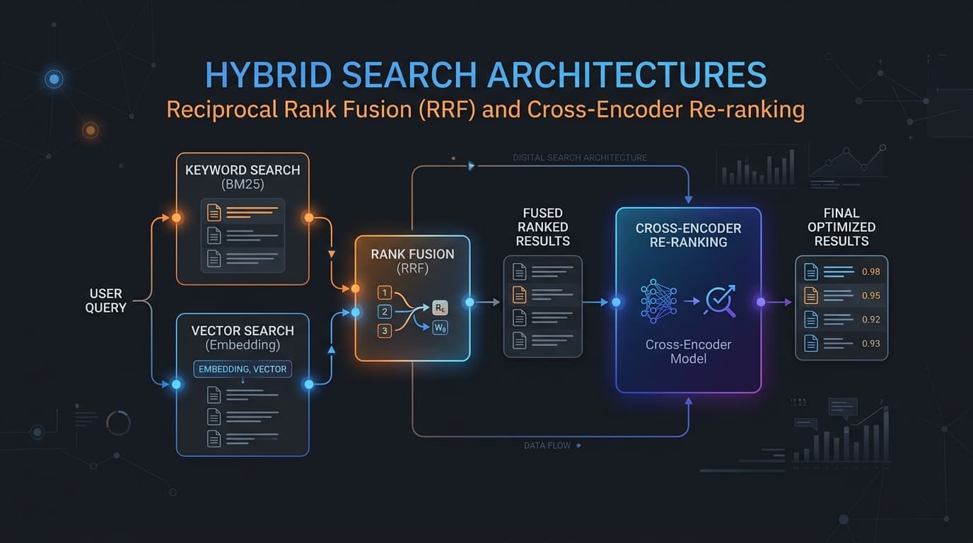
To achieve production-grade accuracy, modern AI engineering has coalesced around a multi-stage retrieval pattern: Hybrid Search combining dense and sparse retrieval, fused via Reciprocal Rank Fusion (RRF), and refined using a Cross-Encoder Reranker. This architecture ensures that the downstream LLM receives the most relevant, contextually complete information while minimizing retrieval latency and compute costs.
What Is It?
A hybrid search architecture is a multi-layered retrieval system designed to maximize both query recall and precision. Instead of relying on a single retrieval mechanism, it processes a query through two parallel pathways and then passes the combined results through a deep-learning re-ranking pipeline:
- Sparse Lexical Retrieval: Utilizing term-matching algorithms such as BM25 (Best Matching 25) to identify documents containing exact keywords, phrases, codes, or identifiers.
- Dense Semantic Retrieval: Utilizing bi-encoder embedding models to map queries and documents into a shared vector space, capturing semantic similarity based on vector distance metrics like cosine similarity or inner product.
- Reciprocal Rank Fusion (RRF): A score-free ranking algorithm that combines the ranked results from both sparse and dense retrieval systems into a single, unified list. RRF is particularly valuable because it evaluates items based on their relative rank in each retrieval list rather than their raw scores, bypassing the need to normalize incompatible scoring metrics (such as BM25 scores versus cosine similarity).
- Cross-Encoder Re-ranking: A high-precision, transformer-based second-stage scoring model. Unlike bi-encoders, which generate separate vector representations for queries and documents, a Cross-Encoder processes the query and document together, allowing full self-attention across all tokens. This captures rich token-to-token interactions to compute a highly accurate relevance score for a subset of candidate documents.
Why It Matters
Implementing a hybrid search architecture with RRF and a Cross-Encoder is not merely an incremental optimization; it is a fundamental requirement for enterprise RAG applications. Without this multi-stage approach, retrieval failures directly translate to LLM hallucinations, incorrect outputs, and user dissatisfaction.
In real-world deployments, keyword matches are often non-negotiable. For instance, if a user queries a technical database for Model-XYZ v2.1.4, a dense vector search might retrieve documents discussing Model-XYZ v2.1.3 or Model-ABC because their semantic profiles are highly similar in embedding space. However, in technical support, retrieving the wrong version's documentation makes the answer useless. BM25 catches this exact token match immediately.
At the same time, lexical search fails when queries are phrased conceptually. If a user asks "How do I speed up query latency when my index blocks writes?", BM25 might fail if the document uses terms like "write locks," "concurrent updates," or "index thrashing" instead of "speed up" or "query latency". Semantic search bridges this conceptual gap.
Optimizing this retrieval pipeline also has profound downstream effects on model serving efficiency. When we supply cleaner, more relevant contexts, we reduce the total prompt length. As we explore in our deep dives on Mitigating Attention Bottlenecks with FlashAttention and Continuous Batching vs PagedAttention, context window length is the single greatest driver of KV-cache size and attention overhead. Serving bloated prompts with irrelevant pages degrades throughput and wastes expensive GPU VRAM. Similarly, if you are serving fine-tuned models optimized via Parameter-Efficient Fine-Tuning (PEFT/LoRA), highly precise retrieval is required to prevent the model from drifting or hallucinating under noisy inputs.
For a deeper dive on how to structure document chunks before indexing them for hybrid search, read our article on Advanced RAG: Hierarchical Node Parsing, Parent-Child Retrievers, and Metadata Pre-Filtering.
How It Works
To understand the mechanics of this architecture, we must analyze the two-stage retrieval and fusion math behind each component.
1. Sparse Lexical Search (BM25)
The BM25 algorithm computes the relevance of a query term q_i to a document d based on term frequency (TF), document length normalization, and inverse document frequency (IDF). Unlike simple TF-IDF, BM25 caps the impact of term frequency so that a keyword appearing 100 times in a document does not make it 100 times more relevant than a document where it appears 5 times.
The formula for BM25 score calculation is:
BM25_Score(D, Q) = sum_{i=1}^{n} IDF(q_i) * [ (f(q_i, D) * (k1 + 1)) / (f(q_i, D) + k1 * (1 - b + b * (|D| / avgdl))) ]
Where:
f(q_i, D)is the term frequency of query tokenq_iin documentD.|D|is the length of documentDin words.avgdlis the average document length across the entire index.k1is a scaling parameter controlling term frequency saturation (typically configured between1.2and2.0).bis a parameter controlling document length normalization (typically configured around0.75).IDF(q_i)is the inverse document frequency of the term, measuring how rare the term is across all documents:
IDF(q_i) = ln( (N - n(q_i) + 0.5) / (n(q_i) + 0.5) + 1 )
Here, N is the total number of documents in the corpus, and n(q_i) is the number of documents containing the term q_i.
2. Dense Semantic Search (Bi-Encoder embeddings)
In dense retrieval, the query q and document d are encoded separately into low-dimensional vectors v_q and v_d (typically 768 or 1536 dimensions) using a transformer-based Bi-Encoder model (such as OpenAI's text-embedding-3 or BAAI's bge-large-en-v1.5).
The similarity score is computed as:
Similarity(q, d) = v_q . v_d / (||v_q|| * ||v_d||)
This dense approach is highly scalable because the document embeddings can be pre-computed and stored in a vector index (e.g., HNSW or IVF-PQ). At query time, the system only needs to embed the query q once and run a fast Approximate Nearest Neighbor (ANN) search.
3. Reciprocal Rank Fusion (RRF)
Because BM25 scores (typically raw floating-point numbers ranging from 0 to 30+) and dense vector similarity scores (typically ranging from 0.0 to 1.0) are calculated using completely different math, they cannot be directly added or multiplied. Normalizing them is notoriously fragile because score distributions change wildly depending on query length and database size.
Reciprocal Rank Fusion (RRF) bypasses this problem entirely. It discards the raw scores and evaluates only the rank (position) of each document in the respective result lists.
The mathematical formula for the RRF score of a document d is:
RRF_Score(d in D) = sum_{m in M} ( 1 / (k + rank_m(d)) )
Where:
Mis the set of retrieval channels (typicallyM = {BM25, Dense_Vector}).rank_m(d)is the rank of documentdin the retrieval systemm(1-indexed). If a document does not appear in a system's top retrieval list, its rank is considered infinite, resulting in a score contribution of0.kis a constant smoothing parameter (traditionally set to60). This constant prevents documents ranked highly in only one list from overwhelming the combined score, while ensuring documents that appear consistently in the top ranks of both lists bubble up.
4. Cross-Encoder Re-ranking
Once the RRF step has merged the results and selected the top candidates (e.g., Top 50), it passes them to the Cross-Encoder.
Unlike a Bi-Encoder which encodes query and document independently, a Cross-Encoder takes both the query and document text concatenated together as a single input sequence:
Input = [CLS] + Query_Text + [SEP] + Document_Text + [SEP]
The sequence is processed through the self-attention layers of a unified transformer network. Every query token is compared directly with every document token, capturing complex semantic dependencies, negative phrasing, qualifiers, and exact contextual matching. A classification head (a Multi-Layer Perceptron) is applied to the output of the [CLS] token to yield a single probability score representing the document's relevance:
Relevance_Score(q, d) = Sigmoid( MLP( Transformer_Output( [CLS] ) ) )
While this process is computationally expensive (and thus unsuitable for scanning millions of documents), it provides unmatched precision when restricted to the top candidates chosen during the first stage.
The following table summarizes the structural differences between Bi-Encoders and Cross-Encoders:
Table 1: Bi-Encoder vs. Cross-Encoder Architecture
| Architectural Feature | Bi-Encoder (Embedding Models) | Cross-Encoder (Reranker Models) |
|---|---|---|
| Input Processing | Query and document encoded separately | Query and document concatenated together |
| Attention Mechanism | No attention between query and document tokens | Full self-attention across query and document |
| Pre-computation | Document embeddings are pre-computed offline | Cannot pre-compute; must process at runtime |
| Computational Complexity | O(1) query-time encoding + fast vector search | O(N) query-time transformer inference passes |
| Primary Metric | Cosine similarity or inner product | Probability score output by classification head |
| Typical Use Case | Candidate retrieval over large databases | High-precision re-ranking of top candidate lists |
Architecture
A robust, enterprise-grade hybrid retrieval architecture is divided into two sequential stages: Stage 1 (High-Recall Candidate Selection) and Stage 2 (High-Precision Re-ranking).
Below is the conceptual flow of a query processing through the pipeline:
graph TD
    User([User Query]) --> PreFilter[Metadata Pre-Filtering]
    PreFilter --> DenseBranch[Dense Retrieval Branch<br/>Bi-Encoder Embedded Query]
    PreFilter --> SparseBranch[Sparse Retrieval Branch<br/>BM25 Lexical Index]

    DenseBranch --> DenseResults[Top-100 Vector Results<br/>Ranked by Cosine Similarity]
    SparseBranch --> SparseResults[Top-100 BM25 Results<br/>Ranked by Term Match Score]

    DenseResults --> RRF[Reciprocal Rank Fusion<br/>RRF score computation with k=60]
    SparseResults --> RRF

    RRF --> CombinedCandidates[Fused Candidates List<br/>Sorted by RRF score]
    CombinedCandidates --> Truncate[Truncate to Top-50 candidates]

    Truncate --> CrossEncoder[Stage 2: Cross-Encoder Reranker<br/>Full Query-Document Self-Attention]
    CrossEncoder --> FinalRerank[Re-ordered Final Candidates List<br/>Ranked by Cross-Encoder Score]

    FinalRerank --> LLMInput[Truncate to Top-5 contexts]
    LLMInput --> LLM([LLM Synthesis Engine])
The pipeline operates as follows:
- User Query & Pre-filtering: The incoming query is normalized. If metadata conditions exist (such as date boundaries or organization IDs), a strict pre-filtering database pass is executed to restrict the search space.
- Parallel Stage 1 Retrieval:
- The query is sent to the dense vector index to execute an approximate nearest neighbor (ANN) search, returning the top 100 documents ranked by semantic similarity.
- In parallel, the query is analyzed by a sparse BM25 engine to search the lexical index, returning the top 100 documents ranked by term matching.
- Rank Fusion: The RRF engine processes both lists. It extracts unique document IDs and calculates an unified RRF score. The documents are sorted by this new score, and the list is truncated to the top 50 candidates.
- Stage 2 Re-ranking: The 50 candidates are paired with the query text and processed in batches by the Cross-Encoder model. The model computes an exact relevance score for each query-document pair.
- Final Output: The list is sorted in descending order of the Cross-Encoder scores. The top 5 documents are selected and formatted into the prompt template passed to the LLM.
Let's look at the latency and compute profiles across these stages:
Table 2: Pipeline Stage Latency and Compute Characteristics
| Pipeline Stage | Algorithm / Model | Latency (Typical) | Memory Profile | Primary Goal |
|---|---|---|---|---|
| Stage 1: Sparse | BM25 (Inverted Index) | 2ms - 10ms | Low (RAM/Disk-bound) | Exact-match keyword recall |
| Stage 1: Dense | Bi-Encoder + Vector Index | 10ms - 25ms | Medium (HNSW index in RAM) | Conceptual semantic recall |
| Stage 1 Fusion | RRF (Smoothing k = 60) | < 1ms | Low (Microsecond CPU compute) | Channel combination |
| Stage 2: Rerank | Cross-Encoder (Transformer) | 150ms - 350ms | High (Requires GPU VRAM) | Document re-ordering precision |
| LLM Generation | Autoregressive LLM | 500ms - 2000ms | Extremely High (VRAM / KV-Cache) | Natural language answer synthesis |
Production Deployment Considerations
Deploying a hybrid retrieval pipeline in production requires balancing operational complexity, query latency, hardware costs, and database capabilities.
1. Database Infrastructure: pgvector vs. Weaviate
Selecting the underlying database dictates how much custom orchestration you must write.
- pgvector (PostgreSQL): If your application already runs on PostgreSQL, pgvector is an operationally simple solution. It allows you to keep relational data and vectors in the same database. However, pgvector does not support native RRF or hybrid search out of the box. You must write custom SQL queries that combine PostgreSQL Full-Text Search (using
tsvectorandtsquery) with pgvector's vector operators (<=>for cosine distance), execute the rank mapping, and calculate the RRF score using custom database functions or application-layer code. - Weaviate: Weaviate is a specialized vector database built natively for hybrid search. It supports native hybrid search queries in a single API call, automatically handling the parallel BM25 and vector queries, executing the RRF merge, and returning the unified ranks. It also supports automated vector indexing and keyword tokenization.
2. Reranker Deployment: Cloud APIs vs. Self-Hosting
Rerankers can be accessed via hosted endpoints or deployed locally:
- Hosted Reranking APIs (e.g., Cohere Rerank v3.5, Jina Reranker v3): These options are highly optimized and handle scale automatically. They provide state-of-the-art accuracy and support features like multilingual inputs and token lengths up to 4096 or 8192 tokens. The drawback is that they introduce network latency and cost money per query.
- Self-Hosted Models (e.g.,
BAAI/bge-reranker-v2-m3): Running an open-weights model within your private VPC guarantees data privacy and eliminates external API costs. However, they must run on GPUs to maintain acceptable query latency (under 200ms). Under high query volume (QPS), you must configure load balancing and batching mechanisms.
The following table compares leading reranking models and options available in 2026:
Table 3: Comparison of Leading Reranker Deployments in 2026
| Reranker Model / API | Deployment Type | Latency (Typical) | Context Window | Key Strengths | Primary Weaknesses |
|---|---|---|---|---|---|
| Cohere Rerank v3.5 | Managed API | 200ms - 350ms | 4096 tokens | Industry-leading accuracy; excellent multilingual support | Pay-per-query pricing; external API dependency |
| Jina Reranker v3 | Managed API / Weights | 180ms - 300ms | 8192 tokens | Listwise reranking; large context window; high precision | Self-hosting is complex; network overhead for APIs |
| BGE Reranker v2-m3 | Self-Hosted | 100ms - 200ms (GPU) | 512 - 1024 tokens | Zero external API costs; full data privacy; open weights | Requires dedicated GPU infrastructure; shorter context window |
| Local BERT-Reranker | Self-Hosted | 50ms - 100ms (GPU/CPU) | 512 tokens | Fast latency; light footprint | Lower retrieval accuracy (NDCG@10) on complex queries |
Common Mistakes
When implementing this architecture, engineers frequently fall into several common traps:
- Reranking Too Many Candidates: A major performance bottleneck is passing large candidate lists (e.g.,
N > 100documents) to the Cross-Encoder. Because Cross-Encoder latency scales linearly with the number of query-document pairs, this can add hundreds of milliseconds of latency, causing query timeouts under high traffic. Keep the reranker input size bounded toN <= 50. - Missing Metadata Pre-filtering: Executing hybrid search and reranking before applying metadata filters is a classic error. If you retrieve the top 50 documents and then filter out those that are outdated, you may be left with only 1 or 2 matching documents. Always apply strict database-level pre-filtering (e.g., SQL
WHEREclauses or vector DB metadata conditions) during Stage 1 retrieval, not after. - Hardcoding the RRF Constant: Using the default
k = 60constant without validating your search corpus is an oversight. If your Stage 1 retrieval returns short, highly precise result lists (e.g., only 5 to 10 candidates),k = 60will flatten the scores, reducing the impact of high-ranking documents. - Running Cross-Encoders on CPUs in Production: While small transformer models can run on CPUs during development, deploying self-hosted rerankers on CPUs under production workloads will lead to high latency. A standard Cross-Encoder like BGE will take over 800ms to rerank 50 documents on standard CPU cores, compared to under 150ms on an Nvidia T4 or L4 GPU.
- Ignoring Score Instability across Models: Trying to compare raw Cosine Similarity scores directly with BM25 scores without using RRF is a common mistake. Because similarity scores shift based on the embedding model's dimensions and training distribution, simple arithmetic merging will inevitably break when models are updated.
Lessons From Production Deployments
Operating hybrid search and reranking systems at scale reveals several critical patterns:
- Implementing Circuit Breakers for Reranking APIs: Hosted reranking APIs can experience transient slowdowns or service outages. Production systems should implement a circuit breaker: if the Cross-Encoder API call fails or times out (e.g., takes longer than 250ms), the system should fail over to the raw RRF ranking list. This ensures that the application remains functional, even if search relevance drops slightly.
- Managing GPU Batching & Concurrency: When self-hosting Cross-Encoders, a surge in user queries can overload the GPU, causing severe latency queues. Implementing query batching (combining document pairs from multiple user requests into a single GPU tensor forward pass) is essential. Deploying models using serving frameworks like Triton Inference Server or vLLM helps manage these concurrent loads.
- Silently Broken Hybrid Indexes: In systems where dense vectors and sparse indices are stored in separate systems (e.g., Elasticsearch for BM25 and a separate vector DB for embeddings), document deletion or schema updates can fall out of sync. This results in "ghost" documents that exist in one index but not the other, leading to RRF scoring failures. Storing both sparse and dense indices in a unified system (like Weaviate, pgvector, or OpenSearch) mitigates this sync risk.
What Most Articles Miss
Most introductory guides treat RRF and Cross-Encoders as simple plug-and-play components. However, a mathematical and architectural analysis reveals several subtle behaviors that can undermine retrieval quality if ignored.
1. The Mathematical Interaction of the RRF Constant k
The smoothing parameter k determines the slope of the rank penalty curve. If k is small, the reciprocal value decreases rapidly as rank drops. For example, if k = 5:
- Rank 1 score:
1 / (5 + 1) = 0.166 - Rank 2 score:
1 / (5 + 2) = 0.142(a 14% drop) - Rank 10 score:
1 / (5 + 10) = 0.066(a 60% drop)
In this scenario, documents ranked highly in any single channel will dominate the fused results.
Conversely, if k is large (e.g., k = 120):
- Rank 1 score:
1 / (120 + 1) = 0.00826 - Rank 2 score:
1 / (120 + 2) = 0.00819(a 0.8% drop) - Rank 10 score:
1 / (120 + 10) = 0.00769(a 7% drop)
With a large k, the penalty curve is flattened. RRF transitions from prioritizing "individual channel wins" to prioritizing "consensus". A document that ranks 15th in both BM25 and vector search will outscore a document that ranks 1st in BM25 but fails to appear in the vector results.
2. Pointwise vs. Listwise Reranking Models
Traditional Cross-Encoders are pointwise models: they score each query-document pair independently. This approach has a fundamental limitation: it ignores the context of the other documents in the candidate pool.
Emerging listwise rerankers (such as Jina Reranker v3) address this by processing multiple document candidates simultaneously. Using listwise attention, the model evaluates how document candidates relate to each other in context. This helps filter out redundant information or group complementary documents, resulting in a cleaner context set for the LLM.
3. Document Length Bias in BM25
The BM25 algorithm includes a document length normalization parameter b. However, in databases containing mixed content (e.g., short 100-token summaries and long 2000-token pages), BM25 often struggles to balance them fairly.
Because sparse retrieval models evaluate term frequency, long documents naturally have more opportunities to match search keywords. Although BM25 normalizes for document length, it still tends to rank long documents higher. When RRF merges these results, the fused ranking can inherit this length bias, pushing short, precise semantic matches down the list. If you notice this pattern, you can tune BM25's b parameter closer to 1.0 to penalize document length more heavily.
Best Practices
To build a reliable and fast hybrid search pipeline, adopt the following engineering practices:
1. Bounded Candidate Set Sizes
Keep the number of candidates passed to the rerank stage small:
- Retrieve the Top 50 to 100 documents from BM25 and Vector search.
- Run RRF and truncate the combined list to the Top 30 to 50 documents.
- Pass only these Top 30 to 50 documents to the Cross-Encoder.
- Pass the final Top 3 to 5 reranked documents to the LLM.
2. Model Quantization for Self-Hosted Deployments
If you self-host Cross-Encoders (like BGE), convert the model weights to FP16, FP8, or INT8 format. Using quantization tools like TensorRT-LLM or ONNX Runtime can reduce inference latency by 30% to 50% and double GPU throughput, allowing you to run rerankers on more affordable hardware.
3. Asynchronous Stage 1 Execution
Ensure the BM25 and vector searches are executed concurrently. In languages like Python, use asyncio to run these database queries in parallel. This prevents the total Stage 1 latency from being the sum of both queries, keeping it bounded to the slower of the two (typically the vector search).
4. Dynamic Candidate Tuning
Adjust the candidate pool size dynamically based on query characteristics. For simple search terms (which contain few words and yield high vector similarity scores), you can reduce the reranker candidate pool to 20 documents. For complex, multi-sentence queries, expand the candidate pool to 50 documents to allow the Cross-Encoder to parse the semantic nuances.
Code Implementation: Orchestrating the Pipeline in Python
Here is a complete, production-ready implementation of a hybrid retrieval pipeline in Python. It demonstrates how to perform parallel Stage 1 search, merge the ranks using RRF, and apply a Cross-Encoder rerank using sentence-transformers.
import asyncio
from typing import List, Dict, Any, Tuple
from rank_bm25 import BM25Okapi
from sentence_transformers import CrossEncoder

class HybridRetrievalPipeline:
    def __init__(self, corpus: List[Dict[str, Any]], rrf_k: int = 60, rerank_top_n: int = 30):
        """
        Initializes the pipeline with a document corpus and tuning configurations.
        """
        self.corpus = corpus
        self.rrf_k = rrf_k
        self.rerank_top_n = rerank_top_n

        # Initialize BM25 lexical search index
        tokenized_corpus = [doc["text"].lower().split(" ") for doc in self.corpus]
        self.bm25 = BM25Okapi(tokenized_corpus)

        # Initialize Cross-Encoder model (self-hosted)
        self.reranker = CrossEncoder("BAAI/bge-reranker-base")

    async def _search_bm25(self, query: str, top_k: int) -> List[Tuple[int, float]]:
        """
        Executes sparse lexical search using BM25.
        Returns a list of tuples containing (document_index, raw_score).
        """
        tokenized_query = query.lower().split(" ")
        scores = self.bm25.get_scores(tokenized_query)
        # Sort documents by score descending and take top_k
        ranked_indices = sorted(enumerate(scores), key=lambda x: x[1], reverse=True)[:top_k]
        return ranked_indices

    async def _search_vector(self, query: str, top_k: int) -> List[Tuple[int, float]]:
        """
        Mock Vector Search for demonstration. In production, this method queries
        a database like Weaviate or pgvector using approximate nearest neighbors (ANN).
        """
        # Simulate small network/index latency
        await asyncio.sleep(0.015)
        # Returns mock document index and dummy cosine similarity scores
        return [(i, 0.85 - (i * 0.005)) for i in range(min(top_k, len(self.corpus)))]

    def _apply_rrf(self, bm25_ranks: List[int], vector_ranks: List[int]) -> List[Tuple[int, float]]:
        """
        Combines sparse and dense ranks using Reciprocal Rank Fusion (RRF).
        """
        rrf_scores: Dict[int, float] = {}

        # Process BM25 ranks
        for rank, doc_idx in enumerate(bm25_ranks):
            # rank is 0-indexed, so we add 1 for 1-based indexing
            rrf_scores[doc_idx] = rrf_scores.get(doc_idx, 0.0) + (1.0 / (self.rrf_k + (rank + 1)))

        # Process Vector ranks
        for rank, doc_idx in enumerate(vector_ranks):
            rrf_scores[doc_idx] = rrf_scores.get(doc_idx, 0.0) + (1.0 / (self.rrf_k + (rank + 1)))

        # Sort documents by final RRF score descending
        sorted_rrf = sorted(rrf_scores.items(), key=lambda x: x[1], reverse=True)
        return sorted_rrf

    async def retrieve(self, query: str, top_k_final: int = 5) -> List[Dict[str, Any]]:
        """
        Orchestrates parallel search, RRF fusion, and Cross-Encoder re-ranking.
        """
        # Run parallel Stage 1 sparse and dense searches
        bm25_task = self._search_bm25(query, top_k=100)
        vector_task = self._search_vector(query, top_k=100)

        bm25_results, vector_results = await asyncio.gather(bm25_task, vector_task)

        # Extract indices in order of rank
        bm25_ranks = [idx for idx, _ in bm25_results]
        vector_ranks = [idx for idx, _ in vector_results]

        # Apply Reciprocal Rank Fusion (RRF)
        fused_results = self._apply_rrf(bm25_ranks, vector_ranks)

        # Truncate to top_n candidates for the reranker
        candidates_to_rerank = fused_results[:self.rerank_top_n]

        if not candidates_to_rerank:
            return []

        # Prepare inputs for Cross-Encoder
        pairs = [(query, self.corpus[doc_idx]["text"]) for doc_idx, _ in candidates_to_rerank]

        # Run inference using the Cross-Encoder model
        rerank_scores = self.reranker.predict(pairs)

        # Map scores back to original documents
        final_rankings = []
        for i, score in enumerate(rerank_scores):
            doc_idx = candidates_to_rerank[i][0]
            final_rankings.append((doc_idx, score))

        # Sort by Cross-Encoder score descending
        final_rankings = sorted(final_rankings, key=lambda x: x[1], reverse=True)

        # Fetch the complete document payloads for the top K results
        top_docs = [self.corpus[doc_idx] for doc_idx, _ in final_rankings[:top_k_final]]
        return top_docs

# Example Usage:
# corpus = [{"id": 1, "text": "Deploying hybrid search with pgvector"}, ...]
# pipeline = HybridRetrievalPipeline(corpus)
# results = asyncio.run(pipeline.retrieve("hybrid search using pgvector"))
FAQ
Here are answers to the most common questions regarding hybrid search, RRF, and Cross-Encoder re-ranking:
1. What is the difference between a Bi-Encoder and a Cross-Encoder?
A Bi-Encoder processes the query and documents independently to generate separate embeddings, allowing you to pre-compute document vectors and execute fast searches. A Cross-Encoder processes the query and document concatenated together in a single transformer pass, enabling token-to-token attention. This makes Cross-Encoders far more accurate but computationally heavier than Bi-Encoders.
2. Why do we need Reciprocal Rank Fusion (RRF) in hybrid search?
BM25 and vector search calculate scores using different scales (e.g., BM25 scores can range from 0 to 30+, while cosine similarity scores range from 0.0 to 1.0). Normalizing these scores is fragile because their distributions vary. RRF avoids this issue by combining the ranks of the documents instead of their raw scores.
3. How do you tune the constant k in the RRF formula?
The constant k (default 60) controls how much weight is given to top-ranked documents. A small k (e.g., 5) prioritizes documents that rank near the top of either list, while a large k (e.g., 100) rewards documents that appear consistently across both lists, smoothing out rank penalties.
4. What is the typical latency of a Cross-Encoder reranker in production?
When running on an enterprise GPU (such as an Nvidia T4 or L4), a Cross-Encoder takes between 100ms and 250ms to score 30 to 50 document candidates. Running the same model on standard CPUs will increase latency to 800ms or more, which can cause timeout issues under heavy traffic.
5. Can pgvector support hybrid search out of the box?
No, pgvector does not have built-in hybrid search or RRF. To build a hybrid pipeline with pgvector, you must query PostgreSQL's native Full-Text Search (using tsvector and tsquery) and pgvector's vector similarity index in parallel, and then merge the results in your application layer or using custom SQL procedures.
6. How does Weaviate implement hybrid search and RRF?
Weaviate supports hybrid search natively. When you run a hybrid query, Weaviate executes vector search and BM25 queries in parallel, applies the RRF algorithm to merge the results, and returns the unified rankings in a single API response.
7. What are the best open-weights reranking models in 2026?
The leading open-weights models are the BGE Reranker series (such as BAAI/bge-reranker-v2-m3 or bge-reranker-large) and the Jina Reranker models. These models offer strong retrieval precision and can be self-hosted on private GPU nodes.
8. When should I use Cohere Rerank API instead of self-hosting BGE?
Use Cohere Rerank v3.5 if you want a managed, highly accurate solution with minimal engineering effort. Host an open-weights model like BGE if you have strict data privacy requirements, or if your application handles very high query volumes where per-query API costs would be too high.
9. Does hybrid search solve the out-of-vocabulary (OOV) problem?
Yes. When a query contains a brand-new term (like a new product ID or serial number) that the vector model was not trained on, the dense vector search may fail. The BM25 sparse search branch will catch the exact keyword match, preserving retrieval accuracy.
10. How does the context window of a reranker impact RAG system costs?
If a reranker has a short context window (e.g., 512 tokens), you must truncate document chunks before scoring them. Models with larger context windows (such as Jina Reranker v3 with 8192 tokens) can score longer documents, but this requires more GPU memory and processing time.
Key Takeaways
- Hybrid retrieval (Vector + BM25) is the industry standard for production RAG systems. It combines the contextual understanding of vector search with the exact keyword-matching capabilities of lexical search.
- RRF simplifies list fusion because it relies on document ranks rather than raw scores, avoiding the fragile math of score normalization.
- Cross-Encoders provide a second-stage accuracy boost (often adding 5 to 15 points in NDCG@10 metrics) by running full self-attention across the concatenated query and document text.
- Keep candidate lists bounded by passing only 30 to 50 documents to the Cross-Encoder. This keeps query latency low and prevents performance bottlenecks under high traffic.
- Run self-hosted rerankers on GPUs or use managed APIs (such as Cohere or Jina) to ensure production queries complete in under 300ms.
