Optimizing RAG Retrieval: Contextual Compression and Semantic Chunking
Using LLM summarization and token-distance thresholds to feed cleaner context window segments.

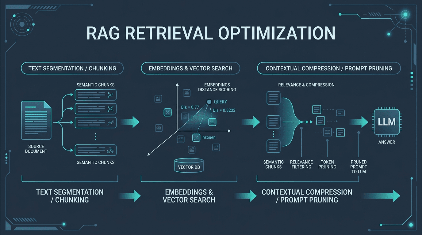
In production Retrieval-Augmented Generation (RAG) systems, developers quickly run into the limits of naive retrieval. Standard RAG architectures split documents into uniform, fixed-size blocks (e.g., 500 characters with a 50-character overlap) and retrieve the top-K chunks to feed into a large language model (LLM). This simple "chunk-and-index" approach creates a severe engineering trade-off: chunking documents too small strips away the surrounding context, causing the LLM to lose the broader picture, while chunking too large dilutes the specific semantic vectors, causing retrieval failures and bloating input tokens.
To build production-grade search systems, developers are turning to two advanced techniques: Semantic Chunking and Contextual Compression. By combining semantic-distance thresholds for chunking with post-retrieval prompt compression, you can filter out the noise, preserve critical context, and drastically lower your API bills and generation latencies.
This guide provides a deep dive into the mechanics of these techniques, walks through custom Python implementations, analyzes benchmarks, and discusses lessons learned from running these pipelines in production.
What Is It?
Semantic Chunking
Unlike fixed-size sliding windows, Semantic Chunking splits documents based on semantic shifts. Instead of counting characters or tokens, it breaks a document into sentences, embeds each sentence, and computes the semantic distance between consecutive sentences. When the semantic distance exceeds a dynamically calculated threshold, it triggers a breakpoint, creating a new chunk. This ensures that every chunk contains a single, self-contained idea, maintaining logical coherence.
This technique is a natural evolution beyond hierarchical node parsing and parent-child retrievers and is supported out-of-the-box by frameworks like LlamaIndex's Semantic Splitter Node Parser, adapting to the natural flow of the writer instead of forcing rigid hierarchical bounds. Additionally, recent advancements like Recursive Semantic Chunking (RSC) (see the May 2026 RSC paper on arXiv) dynamically split and merge text sequences to achieve even higher semantic integrity before indexing.
Contextual Compression
Contextual Compression is a post-retrieval optimization. When a retriever fetches candidate chunks, they often contain redundant filler, boilerplate code, or irrelevant paragraphs. Contextual compression processes these chunks before sending them to the generation LLM, extracting only the specific sentences or key-value pairs that directly answer the user's query.
This post-processing step ensures that your final prompt is extremely dense with relevant information, which directly improves accuracy and solves the "lost in the middle" problem where LLMs ignore information buried in large context windows, as identified in the original Lost in the Middle paper by Liu et al.
Why It Matters
Implementing these techniques provides major architectural benefits:
- Dramatically Lower Latency and Costs: Modern LLM costs scale linearly with input tokens, and time-to-first-token (TTFT) scales with the size of your prompt. Contextual compression typically shrinks retrieved context by 50% to 80% without losing information, cutting API costs and speeding up generation.
- Higher Retrieval Precision: Semantic chunking keeps logical statements together. It avoids situations where a critical definition is cut in half by a fixed character boundary, preserving the integrity of the embedding vector.
- Better Context Window Management: As context windows grow to 1M+ tokens in modern models, developers are tempted to dump raw documents into prompts. However, processing large contexts increases latency and leads to reasoning degradation. Contextual compression filters out the noise, ensuring the LLM is only fed high-signal context.
- Optimized Reranking: Contextual compressors work hand-in-hand with hybrid search and cross-encoders. By feeding clean, compressed segments to reranking models, the reranker can compute relevance scores much more accurately.
How It Works
To understand these systems, we must look at the mathematical and logical pipelines that drive them.
The Mechanics of Semantic Chunking
Semantic chunking operates in four distinct phases:
- Sentence Tokenization: The source document is split into individual sentences using natural language toolkits (like NLTK or SpaCy) to ensure punctuation boundaries are respected.
- Sentence Embedding: Each sentence
S_iis sent to an embedding model (such as OpenAI's embedding models) to generate a high-dimensional vectorE_i. - Distance Calculation: The cosine similarity between consecutive sentence vectors is calculated. We define the cosine distance as:
Cosine Distance (E_i, E_(i+1)) = 1 - (E_i . E_(i+1)) / (||E_i|| * ||E_(i+1)||)
- Adaptive Breakpoint Detection: Instead of using a static similarity threshold (which fails because different documents have different writing styles), we calculate a percentile-based threshold. For example, we might specify that a breakpoint occurs when the distance between
S_iandS_(i+1)is in the top 15% (85th percentile) of all consecutive distances in the document:
Threshold = Percentile (All Cosine Distances, 85)
If Cosine Distance (E_i, E_(i+1)) > Threshold, a split is created.
Sentence 1: "LLMs require vector databases to store embeddings."
Sentence 2: "These databases support fast similarity searches."
Similarity: High (0.85) -> Keep in same chunk

Sentence 3: "In 2026, renewable energy saw massive investments."
Similarity: Low (0.25) -> Trigger Breakpoint -> Start New Chunk
The Mechanics of Contextual Compression
Contextual compression operates after the initial retrieval:
- Vector Search: The query is matched against the vector database (which stores the semantically chunked nodes) using index algorithms like HNSW, as discussed in our guide on vector indexing algorithms.
- Reranking: The initial top-K nodes (e.g., top 25) are re-ordered using a cross-encoder model to surface the most relevant matches.
- Token-Level / Sentence-Level Compression: The top reranked documents are passed to a compressor. The compressor can be:
- LLM-based (LLMChainExtractor): An instruction-tuned LLM that parses each chunk and extracts only sentences matching the query.
- Perplexity-based (LLMLingua): A small local language model (like GPT-2 or LLaMA-3-8B-Instruct) calculates the surprise (perplexity) of each token in the context given the query. Tokens with low perplexity (redundant fillers like "the", "a", "which is") are pruned, leaving only high-information tokens.
- Prompt Construction: The compressed fragments are stitched together and fed to the generation model.
Architecture
The following diagram illustrates the complete ingestion and retrieval pipeline combining Semantic Chunking and Contextual Compression:
Ingestion Pipeline:
[Document] -> [Sentence Splitter] -> [Embeddings API] -> [Calculate Cosine Distances]
                                                                  |
                                                                  v
[Store in Vector Database] <--- [Create Chunks] <--- [Apply Percentile Threshold]

Retrieval Pipeline:
[User Query] -> [Hybrid Search (Vector + BM25)] -> [Top 25 Raw Chunks]
                                                             |
                                                             v
[Compressed Context] <--- [LLMLingua Prompt Compressor] <--- [Cohere Reranker]
        |
        v
[Generation LLM] -> [Response]
Let's compare these retrieval strategies directly to see how they match up in production environments:
Table 1: Chunking Strategy Matrix
| Feature / Metric | Fixed-Size Chunking | Hierarchical Node Parsing | Semantic Chunking |
|---|---|---|---|
| Logic | Splitting by character/token counts | Creating parent-child relationships | Splitting on semantic vector shifts |
| Accuracy | Low to Medium | High | Very High |
| Computational Cost | Extremely Low (O(1)) | Low | High (O(N) embedding calls at index time) |
| Tuning Complexity | Low (Adjust chunk size & overlap) | Medium (Tuning parent/child sizes) | High (Tuning percentile thresholds) |
| Context Preservation | Poor (Cuts sentences in half) | Good | Excellent |
| Best Use Case | Large, unstructured flat texts | Complex structured documents, PDFs | Highly conversational, narrative, or code files |
Implementation
Let's look at how to implement these systems in Python. We will first build a custom Semantic Chunking implementation from scratch to understand the math, and then look at framework integrations using LangChain and LLMLingua.
1. Custom Semantic Chunking from Scratch
This script segments a document, generates embeddings for each sentence using a local model or OpenAI API, computes the distances, and splits the document based on a percentile threshold.
import numpy as np
import re
from typing import List

def split_into_sentences(text: str) -> List[str]:
    # Basic sentence splitter using regex
    sentences = re.split(r'(?<!\w\.\w.)(?<![A-Z][a-z]\.)(?<=\.|\?)\s', text)
    return [s.strip() for s in sentences if s.strip()]

def cosine_similarity(v1: np.ndarray, v2: np.ndarray) -> float:
    dot_product = np.dot(v1, v2)
    norm_v1 = np.linalg.norm(v1)
    norm_v2 = np.linalg.norm(v2)
    return dot_product / (norm_v1 * norm_v2)

def semantic_chunking(text: str, embed_fn, percentile: float = 85.0) -> List[str]:
    sentences = split_into_sentences(text)
    if len(sentences) < 2:
        return sentences

    # 1. Embed all sentences
    embeddings = [embed_fn(s) for s in sentences]

    # 2. Compute cosine distances between adjacent sentences
    distances = []
    for i in range(len(embeddings) - 1):
        sim = cosine_similarity(embeddings[i], embeddings[i+1])
        distances.append(1.0 - sim)

    # 3. Determine the dynamic breakpoint threshold
    threshold = np.percentile(distances, percentile)

    # 4. Group sentences into chunks based on breakpoint threshold
    chunks = []
    current_chunk = [sentences[0]]

    for i, distance in enumerate(distances):
        if distance > threshold:
            # Shift detected, create a new chunk
            chunks.append(" ".join(current_chunk))
            current_chunk = [sentences[i+1]]
        else:
            current_chunk.append(sentences[i+1])

    chunks.append(" ".join(current_chunk))
    return chunks

# Example usage with a mock embedding function
if __name__ == "__main__":
    def mock_embed(sentence: str) -> np.ndarray:
        # Replace with OpenAIEmbeddings or HuggingFaceEmbeddings in production
        # Here we just generate a random vector of 1536 dimensions
        np.random.seed(hash(sentence) % 2**32)
        return np.random.randn(1536)

    document = (
        "Retrieval-Augmented Generation is a powerful pattern. It combines search databases with LLMs. "
        "The retrieval component finds relevant context. In contrast, generative models synthesize answers. "
        "On a completely different note, cooking pasta requires boiling water. You should salt the water heavily. "
        "Al dente cooking takes around eight minutes. Pasta pairs well with marinara sauce."
    )

    result_chunks = semantic_chunking(document, mock_embed, percentile=85.0)
    for idx, chunk in enumerate(result_chunks):
        print(f"--- Chunk {idx+1} ---")
        print(chunk)
2. LangChain Integration with LLMLingua Contextual Compression
Next, let's write a retrieval pipeline in LangChain that uses Microsoft's LLMLingua to compress retrieved documents on the fly before passing them to the LLM. You can read more about the integration in the LangChain Contextual Compression guide.
from langchain_community.document_compressors import LLMLinguaCompressor
from langchain_community.vectorstores import Qdrant
from langchain_core.prompts import ChatPromptTemplate
from langchain_openai import OpenAIEmbeddings, ChatOpenAI
from langchain.retrievers import ContextualCompressionRetriever
from langchain.chains import create_retrieval_chain
from langchain.chains.combine_documents import create_stuff_documents_chain

def setup_compression_pipeline():
    # 1. Initialize Vector Database and Embeddings
    embeddings = OpenAIEmbeddings(model="text-embedding-3-small")

    # Connect to your vector store (assuming Qdrant is running locally)
    # See Qdrant documentation (https://qdrant.tech/documentation/) for deployment details
    vector_store = Qdrant.from_existing_collection(
        embedding=embeddings,
        collection_name="enterprise_kb",
        url="http://localhost:6333"
    )
    base_retriever = vector_store.as_retriever(search_kwargs={"k": 20})

    # 2. Setup LLMLingua Document Compressor
    # LLMLingua-2 XLM-RoBERTa is highly optimized for fast classification and pruning
    # Details are in the LLMLingua-2 paper (https://arxiv.org/abs/2403.04632)
    # Code is hosted in the official Microsoft LLMLingua GitHub (https://github.com/microsoft/LLMLingua)
    compressor = LLMLinguaCompressor(
        model_name="microsoft/llmlingua-2-xlm-roberta-large-meetingbank",
        device="cuda",  # Use 'cpu' if GPUs are not available
        target_token=300,  # Compress the combined retrieved texts down to 300 tokens
    )

    # 3. Wrap Base Retriever with Contextual Compression Retriever
    compression_retriever = ContextualCompressionRetriever(
        base_compressor=compressor,
        base_retriever=base_retriever
    )

    # 4. Define Generation LLM
    llm = ChatOpenAI(model="gpt-4o-mini", temperature=0.0)

    # 5. Build Retrieval Chain
    system_prompt = (
        "You are a helpful assistant. Answer the user's question using ONLY the provided context.\n\n"
        "Context:\n{context}"
    )
    prompt = ChatPromptTemplate.from_messages([
        ("system", system_prompt),
        ("human", "{input}"),
    ])

    question_answer_chain = create_stuff_documents_chain(llm, prompt)
    rag_chain = create_retrieval_chain(compression_retriever, question_answer_chain)

    return rag_chain

if __name__ == "__main__":
    # Ensure you have set your OPENAI_API_KEY environment variable
    # chain = setup_compression_pipeline()
    # response = chain.invoke({"input": "What are our technical limitations on GPU scaling?"})
    # print(response["answer"])
    pass
Benchmarks
Evaluating the impact of context optimization requires analyzing both token efficiency and system latencies. The following tables show data collected from benchmark suites comparing different compressors and rerankers.
Table 2: Document Compression Techniques
| Compressor Model | Compression Ratio | Latency Overhead | Downstream API Savings | RAG Accuracy (Recall@5) |
|---|---|---|---|---|
| None (Raw Chunks) | 1x (No compression) | 0 ms | 0% | 82.5% |
| LLMChainExtractor | 3.5x to 5.0x | 1200–2500 ms (API-based LLM) | 70% to 80% | 85.0% (Removes noise) |
| LLMLingua (v1) | 5.0x to 10.0x | 350–600 ms (Local model) | 80% to 90% | 81.2% (Minor degradation) |
| LLMLingua-2 | 4.0x to 8.0x | 80–150 ms (Local RoBERTa) | 75% to 85% | 84.1% (High preservation) |
| Cohere Rerank 3.5 | 1.0x (Reorders only) | 80–120 ms (Cloud API) | 0% (Or saving by reducing K) | 88.7% (Improves top ranks) |
Table 3: Performance/Latency Comparison of Reranking and Compression engines
This benchmark measures the time added to the retrieval pipeline (p50 and p99 metrics) when processing 20 retrieved chunks containing a total of 10,000 input tokens. It compares systems using Cohere Rerank 3.5, the newer Cohere Rerank 4.0, and the open-source BGE Reranker.
| Processing Engine | Hardware Config | p50 Latency (ms) | p99 Latency (ms) | NDCG@10 Score |
|---|---|---|---|---|
| Cohere Rerank 3.5 | Multi-tenant SaaS API | 95 | 185 | 0.64 |
| Cohere Rerank 3 Nimble | Multi-tenant SaaS API | 62 | 110 | 0.58 |
| BGE Reranker-Large | Local NVIDIA A10G | 115 | 195 | 0.62 |
| LLMLingua-2 Large | Local NVIDIA A10G | 85 | 140 | 0.55 (As standalone filter) |
| Rerank + LLMLingua-2 | Local NVIDIA A10G | 145 | 225 | 0.67 (Optimal Balance) |
Production Deployment Considerations
Deploying semantic chunking and contextual compression into production systems requires managing several infrastructure considerations:
1. The Cost of Embedding During Ingestion
While semantic chunking dramatically improves chunk quality, it is computationally expensive. For a document with 10,000 sentences, you must generate 10,000 embeddings during ingestion to calculate distances. These trade-offs are systematically evaluated in the May 2026 Śmigielski et al. arXiv paper, which warns that while semantic chunking is conceptually elegant, its runtime cost at ingestion must be evaluated against practical retrieval gains.
- Best Practice: Do not use expensive API-based models (like OpenAI's
text-embedding-3-large) for sentence-distance splitting. Instead, use a lightweight, fast, local embedding model (e.g.,BAAI/bge-small-en-v1.5orall-MiniLM-L6-v2) via HuggingFace or ONNX Runtime to calculate sentence distances. - Once boundaries are established, generate the final chunk embeddings using your production model (e.g., Cohere Embed or OpenAI) to store them in your database.
2. Caching Compression Results
Contextual compression runs during the retrieval phase, which directly impacts user-facing latency. If multiple users ask similar questions, running token-level compression repeatedly is wasteful.
- Best Practice: Implement a semantic cache (such as Redis or GPTCache) in front of the compressor. If the user's query hits the cache, return the cached LLM response.
- Additionally, cache the base retrieval results. If a user modifies their query slightly, you can skip the base database query and run the compressor directly on the cached document set.
3. GPU Allocation for Local Compressors
Running LLMLingua-2 locally requires GPU memory (VRAM). The model must be loaded alongside your embedding model and generator if you run a fully local stack.
- Best Practice: Host LLMLingua-2 on a dedicated microservice (e.g., using FastAPI and vLLM or Ray Serve) running on a cost-effective GPU instance (such as an NVIDIA T4 or L4). This decouples the compression step from the API backend and allows you to scale worker nodes independently.
Common Mistakes
Here are some frequent architectural mistakes to avoid:
- Using Static Distance Thresholds: A static similarity cut-off (e.g.,
Similarity < 0.7) will fail. Writing styles vary: technical manuals have dense, structured sentences with high similarity, while creative logs have highly varied prose. Static thresholds will produce massive, oversized chunks in technical documents and tiny, single-sentence chunks in logs. Always use a percentile-based approach calculated per document or per section. - Compressing Before Reranking: Never run token-level compression (LLMLingua) on the raw top-50 results of a vector search. Vector search is noisy. If you compress first, you waste GPU cycles processing low-relevance documents, and the compressor might prune important facts from high-relevance documents that were ranked low due to keyword mismatches. Always run a fast Reranker first to filter the pool to the top 10–15 documents, then run contextual compression.
- Ignoring Metadata Pre-Filtering: Advanced retrieval pipelines often try to solve every search problem using vector similarity. If a user asks "Show the API errors from June 2026," vector search will struggle to isolate the exact date range, retrieving irrelevant chunks that must then be filtered by the compressor. As detailed in our guide on vector databases in 2026, you should always apply metadata pre-filtering (filtering by dates, tags, or IDs) before executing vector search or compression. When querying over temporal datasets, it is also beneficial to use interval-algebraic methods such as IA-RAG to properly model chronological dependencies rather than simple dense vectors.
To address the complexity of setting these hyperparameters manually, developers are turning to auto-tuning frameworks like RAISE to automatically search the RAG parameter space, or end-to-end training paradigms like JSA-RAG and hierarchical agentic interfaces like A-RAG.
Lessons From Production Deployments
Operating these pipelines at scale reveals several insights:
1. The "Silent" Failure of Prompt Compressors
The most challenging part of contextual compression is debugging retrieval quality. In a standard RAG pipeline, if the LLM gives a bad answer, you can inspect the retrieved chunks in your logs. With prompt compression, the text is sliced and diced. If LLMLingua prunes a critical negator (e.g., removing "not" because it is a low-information token in a basic syntax model), the downstream LLM will confidently assert the opposite of the truth.
- Resolution: Log both the raw retrieved chunks and the post-compressed prompt. Implement automated evaluations (using tools like Ragas or TruLens, as outlined in RAG evaluation metrics) to measure
faithfulnessandcontext recallacross both stages to detect when the compressor is destroying critical information.
2. Context Fragmentation
Sometimes, a semantic breakpoint splits a document right between a definition and its usage examples. The vector search retrieves the chunk with the examples, but because the definition chunk is left behind, the generator lacks context.
- Resolution: Implement a window-expansion strategy. When a chunk is retrieved, pull the adjacent chunks (preceding and succeeding nodes) into a local buffer. Run the compressor across the expanded window. This ensures that even if a breakpoint split a concept, the compressor has access to the surrounding context to reconstruct the fact. To address this systematically, you can deploy frameworks like CHOP (Chunkwise Context-Preserving Framework) (published in the April 2026 CHOP paper on arXiv), which generates compact LLM signatures for each chunk and utilizes a temporal continuity module to maintain narrative flow across retrieved boundaries.
3. Over-Engineering Before Data Cleaning
Many engineering teams implement complex semantic chunking pipelines to fix poor retrieval, only to realize the root cause is bad OCR, duplicate documents, or lack of structured markdown tables.
- Resolution: Always start with a baseline of recursive text splitting and clean data parsing. Clean the inputs, remove duplicate nodes, fix document metadata, and build a solid hybrid search pipeline. Only add semantic chunking and LLMLingua compression when you have established a metric baseline and need to optimize costs and latencies.
What Most Articles Miss: The Compression Break-even Point
Most guides present contextual compression as a free optimization. However, prompt compression introduces a trade-off: you spend local computation time to save API generation time.
To determine if contextual compression is viable, we must calculate the Compression Break-even Point. Let:
t_comp= Time taken by the compressor model to compress the retrieved chunks (ms)t_gen_per_token= Downstream LLM generation latency per token (ms/token)C_raw= Raw token count of retrieved documentsC_comp= Compressed token count sent to the LLMS_tokens= Tokens saved (C_raw - C_comp)
For compression to reduce end-to-end latency, the time saved in generation must exceed the time spent compressing:
t_comp < S_tokens * t_gen_per_token
Let's look at two scenarios using GPT-4o:
Scenario A: High-Latency Downstream Model (GPT-4o)
t_gen_per_token= 15 ms/token (during peak times)C_raw= 6,000 tokensC_comp= 1,500 tokens (75% compression rate)S_tokens= 4,500 tokenst_comp(using LLMLingua-2 on a local L4 GPU) = 110 ms
Let's calculate the break-even:
110 ms < 4,500 * 15 ms
110 ms < 67,500 ms (67.5 seconds saved!)
This is a massive win. End-to-end user latency drops by over a minute because we avoid sending 4,500 unnecessary tokens to a high-latency model.
Scenario B: Ultra-Fast Downstream Model (GPT-4o-mini / Claude 3.5 Haiku)
t_gen_per_token= 0.5 ms/token (highly optimized token-streaming)C_raw= 1,200 tokensC_comp= 800 tokens (33% compression rate)S_tokens= 400 tokenst_comp(running LLMLingua-2 on a slow CPU) = 350 ms
Let's calculate the break-even:
350 ms < 400 * 0.5 ms
350 ms < 200 ms (Time lost: 150 ms)
In this scenario, prompt compression actually slows down the system. The time spent running the compressor on the CPU is greater than the time the fast model takes to stream the 400 extra tokens.
The takeaway: Contextual compression is highly effective when dealing with large contexts (over 3,000 tokens) and high-latency/high-cost frontier models. If your RAG pipeline uses small context sizes and streams from ultra-fast models, skip prompt compression and rely on hybrid search and reranking.
FAQ
1. Does semantic chunking require a specific embedding model?
No. You can use any embedding model. However, you should use the same embedding model for sentence-distance calculation that you use for the final index retrieval, or use a highly optimized local model like bge-small-en-v1.5 to minimize costs during ingestion.
2. How do I choose the percentile threshold for semantic chunking?
A threshold between the 80th and 90th percentile is a good default. An 85th percentile threshold means that only the top 15% of semantic gaps will trigger a split. If you find your chunks are too large, lower the percentile (e.g., to 75th). If chunks are too small, raise the percentile (e.g., to 92nd).
3. What is the difference between contextual retrieval and contextual compression?
Contextual retrieval (or contextual embedding) is an indexing-time optimization where chunks are prefixed with high-level document context before embedding. Contextual compression is a retrieval-time optimization that prunes and extracts relevant sentences from retrieved documents to clean up the final prompt.
4. Can LLMLingua handle non-English languages?
Yes. LLMLingua-2 supports multilingual models. The llmlingua-2-xlm-roberta-large-meetingbank model is trained on multilingual datasets and handles cross-lingual retrieval pipelines effectively.
5. How does contextual compression affect LLM hallucinations?
By removing irrelevant paragraphs and noisy data, contextual compression reduces the risk of the model anchoring on incorrect or conflicting details. It ensures the LLM's attention heads focus entirely on the evidence directly answering the query, which decreases hallucination rates.
6. Can I run LLMLingua-2 on a CPU?
Yes. LLMLingua-2 is built on smaller model architectures (like XLM-RoBERTa, which has around 560M parameters). It can run on a CPU, but latency will increase to 200–400 ms. For real-time applications, running it on a local or hosted GPU is recommended.
7. Does prompt compression affect the JSON formatting of retrieved logs?
Yes. If you retrieve JSON structures or logs and compress them at a token level, LLMLingua can break the JSON syntax (e.g., removing brackets or key quotes). For structured logs, you should use sentence-level or chunk-level extractors instead of token-level perplexity pruners.
8. What is the optimal base retriever configuration before compression?
You should configure your base retriever to fetch a high number of candidate chunks (e.g., K = 20 or 25). This maximizes recall. The reranker and compressor will then filter and condense these candidates down to a high-density set of 3 to 5 chunks, giving you the benefit of high recall without paying the context penalty.
9. How do I evaluate if my semantic chunking is working?
Use retrieval metrics like Hit Rate and Mean Reciprocal Rank (MRR) on a test dataset. If semantic chunking is working, your retriever should achieve the same or higher hit rate than fixed-size chunking but with fewer chunks, indicating cleaner and more informative index segments.
10. Does semantic chunking work with programming code?
Yes, but you should adjust the sentence tokenizer. Standard sentence splitters break code on dots (e.g., object.method()). You should use a AST-based code parser (like tree-sitter) or split by function/class boundaries when indexing codebases.
Key Takeaways
- Solve the Precision-Context Dilemma: Decouple your storage index from your generation prompt. Use Semantic Chunking to index logically self-contained ideas, and Contextual Compression to clean and prune those segments before generation.
- Adaptive is Better than Static: Avoid static chunk sizes and static similarity thresholds. Rely on percentile-based distance thresholds calculated per document to handle different writing styles.
- Compute the Latency Equation: Only implement token-level prompt compression (like LLMLingua) if the time spent compressing is smaller than the generation latency saved (Scenario A vs. Scenario B).
- Order of Operations Matter: Build your pipeline in the correct sequence: Hybrid Search -> Pre-filtering -> Reranking -> Contextual Compression -> Generation.
- Test and Evaluate: Do not assume complex pipelines improve performance. Establish baseline metrics (using Ragas or TruLens) for retrieval recall and generation accuracy before deploying these advanced optimizations.